Partial Differential Equations are used in smoothening of images. Under partial differential equations an image is termed as a function; f(x, y), XÎR2. The pixel flux is referred to as an edge stopping function since it ensures that diffusion occurs within the image region but zero at the boundaries; ux(0, y, t) = ux(p, y, t) = uy(x, 0, t) = uy(x, q, t). Nonlinear PDEs tend to adjust the quality of the image, thus giving images desirable outlooks. In the digital world there is need for images to be smoothened for broadcast purposes, medical display of internal organs i.e MRI (Magnetic Resonance Imaging), study of the galaxy, CCTV (Closed Circuit Television) among others. This model inputs optimization in the smoothening of images. The solutions of the diffusion equations were obtained using iterative algorithms i.e. Alternating Direction Implicit (ADI) method, Two-point Explicit Group Successive Over-Relaxation (2-EGSOR) and a successive implementation of these two approaches. These schemes were executed in MATLAB (Matrix Laboratory) subject to an initial condition of a noisy images characterized by pepper noise, Gaussian noise, Brownian noise, Poisson noise etc. As the algorithms were implemented in MATLAB, the smoothing effect reduced at places with possibilities of being boundaries, the parameters Cv (pixel flux), Cf (coefficient of the forcing term), b (the threshold parameter) alongside time t were estimated through optimization. Parameter b maintained the highest value, while Cv exhibited the lowest value implying that diffusion of pixels within the various images i.e. CCTV, MRI & Galaxy was limited to enhance smoothening. On the other hand the threshold parameter (b) took an escalated value across the images translating to a high level of the force responsible for smoothening.
| Published in | Science Journal of Applied Mathematics and Statistics (Volume 12, Issue 1) |
| DOI | 10.11648/j.sjams.20241201.12 |
| Page(s) | 13-19 |
| Creative Commons |
This is an Open Access article, distributed under the terms of the Creative Commons Attribution 4.0 International License (http://creativecommons.org/licenses/by/4.0/), which permits unrestricted use, distribution and reproduction in any medium or format, provided the original work is properly cited. |
| Copyright |
Copyright © The Author(s), 2024. Published by Science Publishing Group |
Partial Differential Equations, Image Processing, Holes, Non-Linear Diffusion Equations, Pixel Flux, Threshold Parameter, Coefficient of the Forcing Term
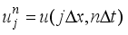
 (1)
(1)  , is a function of the independent variable.
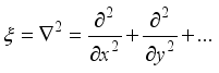
 is a linear operator: For any function
  and
and 
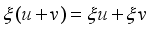 and
and 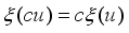 ,
,  is a constant
  . The PDE is inhomogeneous if it has a so called source term:
  , where
  is some function of the independent variables (e.g. Poisson’s equation in electrostatics). Note that one can add solutions of the homogeneous PDE to the inhomogeneous solution. If a PDE is both linear and homogeneous then it obeys the principle of superposition: If
  and
and  are two solutions of a linear, homogeneous PDE, then
  is also a solution, where
  are some constants.
  . At a certain time
  , the value of
  (and possibly its derivative) is identified
  and/or its derivative is determined along a boundary that encloses the region of interest. e.g. electrostatic problems where the potential at the boundaries is specified. In some cases can also have open boundaries.
  ;
; 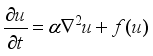 (2)
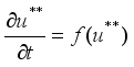
(2)  is the concentration of a substance that is locally generated by a chemical reaction
  , while
  is spreading in space because of diffusion
 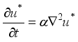 (3)
(3)  (4)
(4)  is a domain in space.
  is a surface and
  . Introducing time
  this image deforms in a partial differential evolution equation (3) according to;
 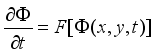 (5)
(5)  is the evolving image [20]
  is an operator that characterizes the given algorithm. The solution of this differential equation gives the processed image at scale
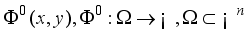
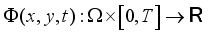
 (6)
(6)  is an unknown function defined in
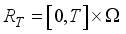
 on
on 
 in
in 
 , the unit normal vector to the boundary of
  . Assuming that
  , a bounded rectangular domain
  , a scaling interval,
  , a non-increasing function,
  is smooth,
  ,
,  , a smoothing kernel (e.g. the Gauss function),
 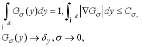 (7)
(7)  is the Dirac measure at the point,
 that enhance the image smoothening process.
  . These values are responsible for smoothening of images that are initially noisy
 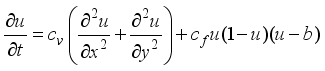 (8)
(8) 2.1. Numerical Approaches
 .
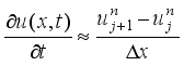
. 2.1.1. Alternating Direction Implicit (ADI) Method
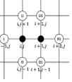
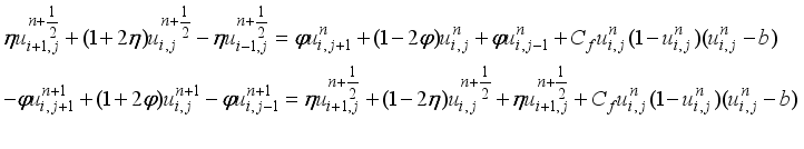 (9)
(9) 2.1.2. Two-Point Explicit Group Successive Over-Relaxation (2-EGSOR)
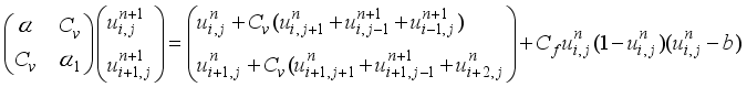 (10)
(10) 2.2. Optimization
 denote a subset of the plane and
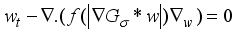
  be a family of gray scale images, and then anisotropic diffusion is defined as;
 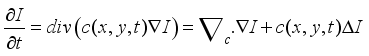 (11)
(11)  , Laplacian
  , gradient
  , divergence operator
  , Diffusion coefficient controls the rate of diffusion
 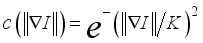 (12)
(12) 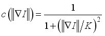 (13)
(13)  Controls the sensitivity to edges and is chosen experimentally or as a function of the noise in the image.
  denote the manifold of smooth images, then the diffusion equations presented above can be interpreted as the gradient descent equations for the minimization of the energy [6] function
  defined by,
 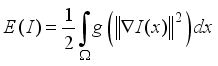 (14)
(14)  is a real-valued function which is intimately related to the diffusion coefficient. Then for any compactly supported infinitely differentiable test function
  ,
,  (15)
(15) 
 denote the gradient of
  with respect to
  the inner product evaluated at
  , this gives;
  (16)
(16)  are given by;
 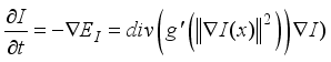 (17)
(17)  the anisotropic diffusion equations are obtained.
  (18)
(18)  , pixel flux
  , Coefficient of theForcing term
  , the threshold parameter
  were applied in the numerical schemes of ADI and 2-EGSOR in MATLAB generating smoothened images.
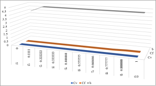
 3.1. Approximated Parameters Under EGSOR
t | Cv | Cf | b |
|---|---|---|---|
0 | 0.000125 | 0.005 | 4 |
0.111111 | 0.00000006968 | 0.006957 | 4.626973 |
0.222222 | 0.00000001597 | 0.007049 | 4.624980 |
0.333333 | 0.0000003090288 | 0.006933 | 4.624997 |
0.444444 | 0.0000002684966 | 0.006931 | 4.624979 |
0.555555 | 0.000000213459 | 0.007012 | 4.624996 |
0.666666 | 0.00000000845238 | 0.006977 | 4.624980 |
0.777777 | 0.00000022759 | 0.006979 | 4.626915 |
0.888888 | 0.00000000882199 | 0.06988 | 4.624981 |
1 | 0.0000000413959 | 0.07018 | 4.624981 |
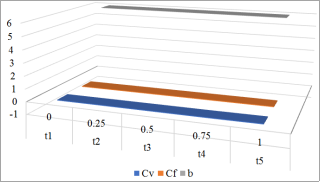
t | Cv | Cf | b |
|---|---|---|---|
0 | 0.000008 | 0.005 | 6 |
0.25 | 0.000000068621 | 0.011784 | 5.999747 |
0.5 | 0.000000256962 | 0.011789 | 5.999747 |
0.75 | 0.0000002491727 | 0.011791 | 5.999743 |
1 | 0.000000157290 | 0.011793 | 5.999752 |
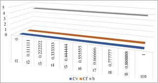
3.2. Approximated Parameters Under ADI
t | Cv | Cf | b |
|---|---|---|---|
0 | 0.000125 | 0.005 | 4 |
0.111111 | 0.000003 | 0.012811 | 4.000023 |
0.222222 | 0.00000045924 | 0.012840 | 4.002498 |
0.333333 | 0.00000002024 | 0.012792 | 4.000023 |
0.444444 | 0.0000000731162 | 0.012818 | 4.002586 |
0.555555 | 0.0000001149168 | 0.012883 | 4.000027 |
0.666666 | 0.0000020747 | 0.012809 | 4.002546 |
0.777777 | 0.0000002403366 | 0.012870 | 4.002569 |
0.888888 | 0.001742 | 0.012647 | 4.000024 |
1 | 0.000745 | 0.012642 | 4.011794 |
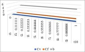
t | Cv | Cf | b |
|---|---|---|---|
0 | -0.000000068622 | 0.011784 | 5.999747 |
0.25 | 0.00196019959 | 0.01607929220 | 5.999766 |
0.5 | 0.00196019959 | 0.01607929220 | 5.999766 |
0.75 | 0.00196019959102 | 0.01607929220 | 5.999766 |
1 | 0.0196019959102702 | 0.01607929220 | 5.999766 |
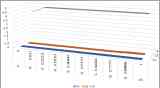
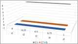
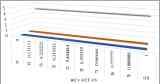
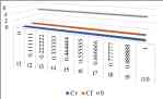
 which is the threshold parameter maintains the highest value as opposed to
  which is the pixel flux, it registers the lowest value implying pixel diffusion is limited in the smoothening process. On the other hand the forcing term coefficient
  is of moderate value, inputing minimum force into the image in the course of smoothening hence limiting blurring.
  ,
,  ,
,  . Parameter
  works best when optimized to the highest value as compared to
  ,
,  . Smoothening of images can be done well when parameters are minimized. I recommend use of other computer programs other than MATLAB in future optimization.
 | [1] | Alvarez, L., Guichard, F., Lions, P. L., Morel, J. M. (1993): Axioms and fundamental equations of image processing. Arch. for Rational Mechanics 123(3), 199–257. |
| [2] | Benson, D. A., Wheatcraft, S. W., and Meerschaert, M. M. (2000). Application of a fractional advection-dispersion equation. Water Resources Research, 36(6): 1403-1412. |
| [3] | Bueno-Orovio, A., Kay D., and Burrage, K. (2012). Fourier spectral methods for fractional in-space reaction-diffusion equations. Journal of Computational Physics. |
| [4] | Caselles, V., and Sbert, C. (1996) What is the best causal scale space for three-dimensional images? SIAM Journal applied mathematics, 56(4): 1119–1246. |
| [5] | Caputo, M. (1967). Linear models of dissipation whose q is almost frequency Independent Geophysical. Journal of the Royal Astronomical Society, 13(5): 529-539. |
| [6] | Cattaneo, C. (1948). Sulla conduzione del calore. Atti Semin. Mat. Fis. Della Universita di Modena, 3: 3. |
| [7] | Chen, Y., Yu, W., and Pock, T. (2015). Learning optimized reaction diffusion processes for effective image restoration. Proceedings of IEEE conference on computer vision and pattern recognition (Boston: IEEE) pp 5261-69. |
| [8] | Caselles, V., Morel, J. M., Sapiro, G., A. Tannenbaum (1998): Special issue on partial differential equations and geometry-driven diffusion in image processing and analysis. IEEE Trans. Image Processing 7(3). |
| [9] | Compte, A., and Metzler, R. (1997). The generalized Cattaneo equation for the description of anomalous transport processes. Journal of Physics A: Mathematical and General, 30: 7277-7289. |
| [10] | Ebihara, M., Mahara, H., Osa, A., and Miike, H. (2003) Segmentation and edge detection of noisy image and low contrast image based on a reaction-diffusion model The Journal of the Institute of Image Electronics Engineers of Japan, 32: 378–385. |
| [11] | Einstein, A. (1905). “die von der molekularkinetischen Theorie der Warme geforderte Bewegung von in ruhenden Flussigkeiten suspendierten Teilchen "Annalen der Physik (in German). 322(8): 549-560. |
| [12] | Gabor, D (1965) Information theory in electron microscopy. Laboratory Investigation 14, 801–807. |
| [13] | Gerbrands, J. J., Schavemaker, J. G. M., Reinders, M. J. T., and Backer, E. (2000). Image Sharpening by morphological filtering, Pattern Recognition, 33: 997–1012. |
| [14] | Gilboa, G., Sochen, N., Zeevi, Y. (2004): Image enhancement and denoising by complex diffusion processes. IEEE Trans. Pattern Analysis and Machine Intelligence 26(8), 1020–1036. |
| [15] | Grégoire, N., and Ana, I. T. M. (2020). “On the maximization problem for solutions of reaction–diffusion equations with respect to their initial data”. In: Mathematical Modelling of Natural Phenomena 15, p. 71. |
| [16] | Haar Romeny, B. M. (1994). Geometry-Driven Diffusion in Computer Vision. Kluwer Academic Publishers. |
| [17] | Jacobs, B. A., and Harley, C. (2013). A comparison of two hybrid methods for solving linear time-fractional partial differential equations on a two-dimensional domain. Sub-mitted to Abstract and Applied Analysis Special Issue: New Trends on Fractional and Functional Differential Equations. |
| [18] | Lee, J. S. (1980). Digital image enhancement and noise filtering by use of local statistics. IEEE Pat. Anal. Mach. Intell., 2: 165–168. |
| [19] | Jumarie, G. (2005). On the solution of the stochastic differential equation of exponential growth driven by fractional Brownian motion. Applied Mathematics Letters, 18: 817-826. |
| [20] | Koenderink, J. (1984) The structure of images. Biological Cybernetics 50, 363–370. |
| [21] | Malladi, R., Sethian, J. A., and Vemuri, B. C. (1995). “Shape modeling with front propagation,” IEEE Trans. Pattern Anal. Machine Intel, vol. 17, pp. 158–175, Feb. |
| [22] | Mumford, D., and Shah, J. (1989). “Optimal approximations by piecewise smooth functions and variation problems,” Commun. Pure Appl. Math., vol. 42. |
| [23] | Oldham, K. B., and Spanier, J. (1974). The Fractional Calculus. Academic Press, Inc. |
| [24] | Osher, S., and Rudin, L. (1990) Feature oriented image enhancement using shock filters. SIAM J. Numerical Analysis, 27: 919–940. |
| [25] | Ozkan, M. K., Sezan, M. I., and Tekalp, A. M. (1993) Adaptive motion compensated filtering of noisy image sequences. IEEE Trans. Circuits and Systems for Video Technology, 3: 277–290. |
| [26] | Peaceman, D. W., and Rachford Jr. H. H. (1955). The numerical solution of parabolic and elliptic differential equations. Journal of the Society for Industrial and Applied Mathematics, 3(1): 28–41. |
| [27] | Perona, P., and Malik, J. (1990). "Scale-space and Edge Detection Using Anisotropic Diffusion," IEEE Transactions on Pattern Analysis and Machine Intelligence, 12(7), pp. 629-639. |
| [28] | Rasmussen, F. S., Sonne M. R., Larsen, M. J., Spangeberg, Lilleheden L. T. and Hattel, J. H.(2018). A characterization study relating cross-sectional distribution of fiber volume fraction and permeability. Proc. 22nd Int. Conf. on Compos. Mater. (Melbourn, Australia). |
| [29] | Sapiro, G. (2001) Geometric Partial Differential Equations and Image Analysis. Cambridge University Press. |
| [30] | J. H. (2017): 2D Numerical Modelling of thge Resin Injection Pultrusion Process Including Experimental Resin Kinetics and Temperature Validation. Proceeding: ICCM21. |
| [31] | Witkin, A. (1983) Scale-space filtering. In: Proc. Int. Joint Conf. Artificial Intelligence. |
APA Style
Fwamba, R. N., Chepkwony, I., Fwamba, W. S. (2024). Optimization of the Non-Linear Diffussion Equations. Science Journal of Applied Mathematics and Statistics, 12(1), 13-19. https://doi.org/10.11648/j.sjams.20241201.12
ACS Style
Fwamba, R. N.; Chepkwony, I.; Fwamba, W. S. Optimization of the Non-Linear Diffussion Equations. Sci. J. Appl. Math. Stat. 2024, 12(1), 13-19. doi: 10.11648/j.sjams.20241201.12
@article{10.11648/j.sjams.20241201.12,
  author = {Rukia Nasimiyu Fwamba and Isaac Chepkwony and Wekulo Saidi Fwamba},
  title = {Optimization of the Non-Linear Diffussion Equations},
  journal = {Science Journal of Applied Mathematics and Statistics},
  volume = {12},
  number = {1},
  pages = {13-19},
  doi = {10.11648/j.sjams.20241201.12},
  url = {https://doi.org/10.11648/j.sjams.20241201.12},
  eprint = {https://article.sciencepublishinggroup.com/pdf/10.11648.j.sjams.20241201.12},
  abstract = {Partial Differential Equations are used in smoothening of images. Under partial differential equations an image is termed as a function; f(x, y), XÎR2. The pixel flux is referred to as an edge stopping function since it ensures that diffusion occurs within the image region but zero at the boundaries; ux(0, y, t) = ux(p, y, t) = uy(x, 0, t) = uy(x, q, t). Nonlinear PDEs tend to adjust the quality of the image, thus giving images desirable outlooks. In the digital world there is need for images to be smoothened for broadcast purposes, medical display of internal organs i.e MRI (Magnetic Resonance Imaging), study of the galaxy, CCTV (Closed Circuit Television) among others. This model inputs optimization in the smoothening of images. The solutions of the diffusion equations were obtained using iterative algorithms i.e. Alternating Direction Implicit (ADI) method, Two-point Explicit Group Successive Over-Relaxation (2-EGSOR) and a successive implementation of these two approaches. These schemes were executed in MATLAB (Matrix Laboratory) subject to an initial condition of a noisy images characterized by pepper noise, Gaussian noise, Brownian noise, Poisson noise etc. As the algorithms were implemented in MATLAB, the smoothing effect reduced at places with possibilities of being boundaries, the parameters Cv (pixel flux), Cf (coefficient of the forcing term), b (the threshold parameter) alongside time t were estimated through optimization. Parameter b maintained the highest value, while Cv exhibited the lowest value implying that diffusion of pixels within the various images i.e. CCTV, MRI & Galaxy was limited to enhance smoothening. On the other hand the threshold parameter (b) took an escalated value across the images translating to a high level of the force responsible for smoothening.},
 year = {2024}
}
TY  - JOUR
T1  - Optimization of the Non-Linear Diffussion Equations
AU  - Rukia Nasimiyu Fwamba
AU  - Isaac Chepkwony
AU  - Wekulo Saidi Fwamba
Y1  - 2024/04/02
PY  - 2024
N1  - https://doi.org/10.11648/j.sjams.20241201.12
DO  - 10.11648/j.sjams.20241201.12
T2  - Science Journal of Applied Mathematics and Statistics
JF  - Science Journal of Applied Mathematics and Statistics
JO  - Science Journal of Applied Mathematics and Statistics
SP  - 13
EP  - 19
PB  - Science Publishing Group
SN  - 2376-9513
UR  - https://doi.org/10.11648/j.sjams.20241201.12
AB  - Partial Differential Equations are used in smoothening of images. Under partial differential equations an image is termed as a function; f(x, y), XÎR2. The pixel flux is referred to as an edge stopping function since it ensures that diffusion occurs within the image region but zero at the boundaries; ux(0, y, t) = ux(p, y, t) = uy(x, 0, t) = uy(x, q, t). Nonlinear PDEs tend to adjust the quality of the image, thus giving images desirable outlooks. In the digital world there is need for images to be smoothened for broadcast purposes, medical display of internal organs i.e MRI (Magnetic Resonance Imaging), study of the galaxy, CCTV (Closed Circuit Television) among others. This model inputs optimization in the smoothening of images. The solutions of the diffusion equations were obtained using iterative algorithms i.e. Alternating Direction Implicit (ADI) method, Two-point Explicit Group Successive Over-Relaxation (2-EGSOR) and a successive implementation of these two approaches. These schemes were executed in MATLAB (Matrix Laboratory) subject to an initial condition of a noisy images characterized by pepper noise, Gaussian noise, Brownian noise, Poisson noise etc. As the algorithms were implemented in MATLAB, the smoothing effect reduced at places with possibilities of being boundaries, the parameters Cv (pixel flux), Cf (coefficient of the forcing term), b (the threshold parameter) alongside time t were estimated through optimization. Parameter b maintained the highest value, while Cv exhibited the lowest value implying that diffusion of pixels within the various images i.e. CCTV, MRI & Galaxy was limited to enhance smoothening. On the other hand the threshold parameter (b) took an escalated value across the images translating to a high level of the force responsible for smoothening.
VL  - 12
IS  - 1
ER  -
Department of Mathematics & Actuarial Science, Kenyatta University, Nairobi, Kenya
Department of Mathematics & Actuarial Science, Kenyatta University, Nairobi, Kenya
Department of Disaster Preparedness and Engineering Management, Masinde Muliro University of Science and Technology, Kakamega, Kenya
Information