The Food and Drug Administration’s 2011 Process Validation Guidance and International Council for Harmonization Quality Guidelines recommend continued process verification (CPV) as a mandatory requirement for pharmaceutical, biopharmaceutical, and other regulated industries. As a part of product life cycle management, after process characterization in stage 1 and process qualification and validation in stage-2, CPV is performed as stage-3 validation during commercial manufacturing. CPV ensures that the process continues to remain within a validated state. CPV requires the collection and analysis of data related to critical quality attributes, critical material attributes, and critical process parameters on a minimum basis. Data is then used to elucidate process control regarding the capability to meet predefined specifications and stability via statistical process control (SPC) tools. In SPC, the control charts and Nelson rules are commonly used throughout the industry to monitor and trend data to ensure that a process remains in control. However, basic control charts are susceptible to false alarms and nuisance alarms. Therefore, it is imperative to understand the assumptions behind control charts and the inherent false alarm rates for different Nelson rules. In this article, the authors have detailed the assumptions behind the usage of control charts, the rate of false alarms for different Nelson rules, the impact of skewness and kurtosis of a data distribution on the false alarm rate, and methods for optimizing control chart design by reducing false alarm rates and nuisance signals.
This is an Open Access article, distributed under the terms of the Creative Commons Attribution 4.0 International License (http://creativecommons.org/licenses/by/4.0/), which permits unrestricted use, distribution and reproduction in any medium or format, provided the original work is properly cited.
CPV, Control Chart False Alarm Rate, Control Chart Skewness and Kurtosis, Control Chart Nuisance Signal
1. Introduction
The Food and Drug Administration (FDA)’s 2011 Process Validation Guidance recommends continued process verification (CPV) during stage-3 process monitoring for drug manufacturers. In CPV, Shewhart control charts are employed as a statistical tool for monitoring process parameters and attributes (critical process parameters (CPPs), Key process parameter (KPPs), In-process controls (IPCs), batch yields, step recovery yields and release specifications). In control charts, the calculated process average is utilized as the center line, and control limits are placed at distance k = ±3 short-term standard deviations (σR) away from the process average. The control chart, along with Nelson rules, serves as a tool for detecting out-of-control (OOC) data, defined as data that fall beyond the set control limits, and out-of-trend (OOT) data, defined as a group of data that forms a non-random pattern (shift in mean or increasing/decreasing pattern)
[1]
Guidance for Industry: Process Validation — General Principles and Practices. US Food and Drug Administration: Silver Spring, MD, 2011;
Heigl, N., Schmelzer, B., Innerbichler, F., & Shivhare, M. (2021). Statistical quality and process control in Biopharmaceutical manufacturing—Practical issues and remedies. PDA Journal of Pharmaceutical Science and Technology, 75(5), 425-444.
. Although control charts are commonly applied across the industry to assess the statistical stability of a process, this approach introduces two types of risk: 1) false alarms, i.e., signals that are incorrectly identified as OOC or OOT when the data are actually belong to normal variability of the process itself, and 2) nuisance alarms, i.e., signals that are too small to have any impact on the process or lack sufficient statistical reliability
[4]
Adams, B. M., Woodall, W. H., & Lowry, C. A. (1992). The use (and misuse) of false alarm probabilities in control chart design. Frontiers in Statistical Quality Control 4, 155-168.
Walker, E., Philpot, J. W., & Clement, J. (1991). False signal rates for the Shewhart control chart with supplementary runs tests. Journal of Quality Technology, 23(3), 247-252.
. In practice, small process variations and shifts are anticipated in many processes; therefore, control charts should detect moderate to large shifts that have more practical application rather than small or practically insignificant shift signals. Both high false alarm rates (FARs) and frequent nuisance alarms will reduce the reliability of control chart signals. Therefore, in this article, we provide a review on the current state of understanding on FARs associated with different Nelson rules, properties of data distributions (skewness and kurtosis) and their impact on control chart FAR, and methods for reducing FARs by optimizing the usage of Nelson rules and adjusting the value of k (the number of standard deviations from the mean) to accommodate variability and asymmetricity in data distribution.
2. Functional Modules of CPV
CPV program is driven by four functional models as identified in Figure 1. CPV standard operating procedure (SOP): Drug manufactures define standard operating procedure for CPV as a guidance document that minimum should discuss 1) criteria for selection parameters to be monitored and trended 2) Frequency of cross functional team to perform data review meeting to monitor and analyze the trends of parameters and attributes, 3) Participants in the cross functional CPV data review meeting, 4) Discuss different statistical methods to assess the process capability and stability based on type of data distribution, 5) Method of controlled way of documenting the meeting minutes of CPV data review meeting, 6) Guidance on frequency of CPV report generation based on batch run rate, and 7) Guidance on reaction and response to signals from CPV data monitoring system.
CPV Plan: As per the recommendations in CPV SOP, CPV plan is generation for each drug substance intermediate stage, that list out all the parameters to be monitored and trended, type of data distribution and statistical method may be applied to assess the stability and capability.
CPV data review meeting: As recommended in the CPV SOP the parameters listed in CPV plans are charted and analyzed for signals of unexpected variation from historical performance as a cross functional team that includes a minimum participation from manufacturing, quality assurance (QA), manufacturing science and technology (MSAT) and quality control (QC). During the data review the identified statistical process control signals for OOT or OOC are disused on; 1. Magnitude of signal, 2. Statistical reliability of signal 3. Risk and severity on product quality or/and process performance, and the decision on how to respond to the signal. If the signal is identified as nascence signal or not practically significant enough or not statistically significant enough, then no response or action is required. If the signal is identified to be real and has both practical and statistical strength but still not significant enough to impact product quality, then a technical evaluation may be warranted to understand the cause of variation, details of evaluation and results should be followed up in subsequent CPV meetings and findings should be documented in CPV meeting minutes. If the signal is identified to be real, has both practical and statistical significance, and the magnitude is significant enough to potentially impact the product quality, then an investigation under quality management system may be required.
CPV reports: CPV reports are generated either annually or semiannually or quarterly basis based on batch run rate. Here all parameters and attributes listed in CPV pans are monitored and trended along with summary stability and capability discussions along with all the CPV data review meeting minutes. Recommendations from the CPV reports may include changes in the frequency of monitoring a parameter, retiring, or adding parameters to CPV plans. CPV plans should be reviewed at least annually and may be revised if required to ensure that the recommended changes from CPV reports are implemented appropriately.
In 1924, Walter Andrew Shewhart introduced the concept of data analysis using control charts, which was later adopted by the pharmaceutical and biopharmaceutical industries when regulatory agencies requested that drug manufacturers to perform CPV
[6]
Nelson, L. S. (1984). The Shewhart control chart—Tests for special causes. Journal of Quality Technology, 16(4), 237-239.
. In control charts or XBar charts, the center line is placed at the average, and control limits are typically placed at k standard deviations from the average. Typically, k = 3 is utilized, for which there is a 0.135% probability that any data point belonging to a normally distributed population will fall outside ±3 standard deviations (σ). This approach gives an interval of expected future observations if the process does not change. If observations are within these limits, it can be assumed that the validated state is maintained; if observations are outside these limits, the mean and/or standard deviation has probably changed, potentially requiring attention. σ is often calculated as a short-term σR, which causes the limits to be more sensitive to drift, as expressed in (1).
(1)
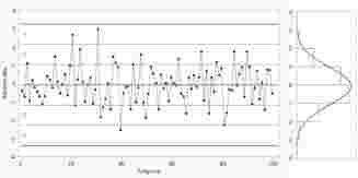
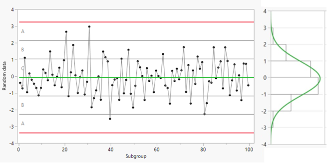
The control chart is divided into six zones based on distance from the center line as shown in Figure 2. Each zone is one standard deviation (σR) wide. The 3-σR limits on both sides of the center line show the upper control limit and lower control limit. The 2-σR limits indicate the upper and lower warning limits, and the 1-σR limits on each side of the center line are the upper and lower one-sigma limits. Control charts, along with Nelson rules 1–8 (summarized in Table 1), are used to monitor process control and process stability based on the location of data in different zones, the frequency of occurrence of any patterns, and the distance from the mean
[6]
Nelson, L. S. (1984). The Shewhart control chart—Tests for special causes. Journal of Quality Technology, 16(4), 237-239.
. To correctly apply the Nelson test rule signals in a control chart, it is imperative to understand the normal acceptable probability for a data point to fall within or outside of the control chart zones. For instance, a hypothetical mean µ=0 and standard deviation σ=1, the probability that normally distributed data will fall between -3 SD and +3 SD is given by (2).
Figure 2. Sample X control chart constructed from randomly generated data.
In statistical process control, the FAR or rate of type I errors, often identified by the symbol α, indicates the likelihood that data will be falsely identified as an abnormal signal when the data correspond to the normal variability of the process. Table 1 summarizes the different Nelson rules and their purposes, along with probability of a false alarm for each Nelson rule
[7]
Griffiths, D., Bunder, M., Gulati, C., & Onizawa, T. (2010). The probability of an out of control signal from Nelson's supplementary zig-zag test. Journal of Statistical Theory and Practice, 4(4), 609-615.
The FARs from all eight Nelson rules identified in Table 1 sum up to 2.65%. Although it might be intriguing to use all eight Nelson test rules, Nelson (1984) suggested keeping the FAR below 1%
[6]
Nelson, L. S. (1984). The Shewhart control chart—Tests for special causes. Journal of Quality Technology, 16(4), 237-239.
. Nelson also stated that tests 5 and 6 should be included only when there is an economical desire to have an early warning, as these test rules increase the FAR by 2%. Tests 7 and 8 are used to diagnose stratifications and both test 7 and 8, react only when each reported results in control charts are from an average of 2 or more samples (i.e. subgroup size “m” ≥ 2). However, in the biopharmaceutical industry, the results reported for a batch is typically from a test performed on single sample; therefore, unless multiple samples are tested and averaged to report a single value in the control chart, rules 7 and 8 do not add value for data monitoring and trending. Adhibhatta et al. (2017) showed that Nelson tests 1, 2, and 3 are adequate for monitoring OOC and OOT data, with a combined false alarm probability of 0.94
[8]
Adhibhatta, S., DiMartino, M., Falcon, R., Haman, E., Legg, K., Payne, R., Pipkins, K., & Zamamiri, A. (2017). Continued process verification (CPV) signal responses in Biopharma. ISPE | International Society for Pharmaceutical Engineering.
. Thus, considering the practical application of test rules for biopharmaceuticals and to limit the FAR below 1.0%. It is recommended that only Nelson test rules 1 to 3 be utilized in a control chart for biopharmaceutical application.
Table 1. FARs for different Nelson test rules.
Test number
Purpose
Probability of false alarm
Rule 1: One data point outside the control limit
Detect OOC data
p = 0.00270
Rule 2: Nine consecutive data points on one side of the centre line
Detect a process shift
p = 0.00391
Rule 3: Six consecutive data points either increasing or decreasing
Detect a process drift
p = 0.00278
Rule 4: Fourteen consecutive data points alternating up and down
Detect a process alternating between two states
p = 0.00457
Rule 5: Two out of three data points falling outside two sigma from the centre line
Detect an intermediate shift
p = 0.00306
Rule 6: Four out of five data points falling outside two sigma from the centre line
Detect a small shift
p = 0.00553
Rule 7: Fifteen data points falling within one sigma from the centre line
Detect a reduction in process variability
p = 0.00326
Rule 8: Eight consecutive data points falling outside one sigma from the centre line
Detect mixed process behaviour
p = 0.00010
4. FAR in an OOC Signal from a Limited Sample Size
OOC data are detected via Nelson rule 1 when a single data point falls outside 3 SD from the mean, with the assumptions that the data are normally distributed, the underlying true population mean (µ) and population standard deviation (σ) are known, and there is no error due to sampling variability. However, for new products, based on the batch run rate, there is a high likelihood of having a very limited sample size during the first couple of years. For small sample sizes, the estimation of the population mean with the sample mean (x̄) and of the population standard deviation with the sample standard deviation (SD) and the establishment of control limits will lead to an increased FAR
[9]
Trietsch, D., & Bishak, D. (2007). The Rate of False Signals for Control Charts with Limits Estimated from Small Samples. Journal of Quality Technology, 39(1), 52-63.
Braden, P., & Matis, T. (2022). Cornish–fisher-based control charts inclusive of skewness and kurtosis measures for monitoring the mean of a process. Symmetry, 14(6), 1176.
. The risk of an increased FAR due to a limited sample size in control limits has been calculated by Bischak et al. (2007) as a function of the number of standard deviations from the mean (k), the number of observations reported in control chart (n), and the size of the subgroup used in each observation (m). As discussed above, biopharmaceutical companies typically perform testing on a single sample taken from a batch; therefore, two subsequent lots are used to calculate the short-term standard deviation, and hence, m is assumed to be 2. The FAR for a limited number of observations or sample size (n) is expressed in (3). Here, (C4) is an unbiased estimator of standard deviation. The uncertainty that arises from using the sample standard deviation (SD) instead of the underlying true population standard deviation is compensated for by using an unbiased standard deviation estimator (C4) calculated as a function of subgroup size, as expressed in (4)
[10]
Bischak, D. P., & Trietsch, D. (2007). The rate of false signals in u control charts with estimated limits. Journal of Quality Technology, 39(1), 54-65.
Munoz, J., Moya Fernandez, P., Alvarez, E., & Blanco-Encomienda, F. (2020). An alternative expression for the constant c4[n] with desirable properties. Scientia Iranica, 0(0), 3388-3393.
. Here, Φ is the cumulative normal probability density function.
(3)
(4)
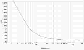
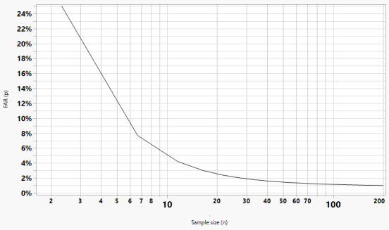
The probability of a false alarm caused by utilizing a limited sample size when setting the control limit at k = 3 (i.e., 3 standard deviations from the mean) is calculated by applying (3) and (4), as shown in Figure 3. Figure 3 shows that the reduction in FAR follows an exponential decay curve; we observe a sharp drop below 5% for a sample size of n = 10, followed by a plateau after approximately n = 30 and a further decrease below 1% at n = 100. Therefore, we recommend using a run chart when the sample size is ≤10, using the calculated control limits as tentative control limits for monitoring and updating control limits for sample sizes of 30–100, and using fixed long-term control limits when the sample size is ≥100. Another alternative solution for mitigating the uncertainty in the calculation of control limits for a small sample size (10 ≤ n < 30) is the use of prediction limits. Prediction limits account for the estimation uncertainty that arises from using the sample standard deviation (SD) by replacing the normal quantile with the t quantile at (n–1) degrees of freedom and also accommodates the uncertainty due to the sample mean by including the standard error of the mean, as expressed in (5).
Figure 3. FAR in an OOC signal from a limited sample size.
5. FAR in an OOC Signal from a Skewed or Heavy-Tailed Distribution
The application of Nelson test rules in a control chart is based on a normality assumption. However, if the data are severely skewed or if the variance in the data is excessively broad with a heavy-tailed distribution, this can lead to an increase in the FAR. The asymmetry and tail length in data with reference to a normal distribution are measured as skewness (K3) and kurtosis (K4), respectively
[14]
Braden, P., & Matis, T. (2022). Cornish–fisher-based control charts inclusive of skewness and kurtosis measures for monitoring the mean of a process. Symmetry, 14(6), 1176.
5.1. Modeling FAR for an Asymmetric Data Distribution
Control charts are based on the assumption that a data distribution is symmetric on either side of the center average line. However, in practice, the data distribution may be off-centered or asymmetric. Skewness (K3) is a measure of the degree of asymmetry observed in a data distribution. A distribution can have either right-skewed or left-skewed data or no skew at all. A right-skewed distribution is longer on the right side of its peak, and a left-skewed distribution is longer on the left side of its peak. Skewness in a distribution can be calculated from (6)
[11]
Richard A. Groeneveld, Glen Meeden, (1984). Measuring Skewness and Kurtosis, Journal of the Royal Statistical Society, 33(4), 391–399,
. A highly skewed distribution can lead to a high FAR in control chart signals. The probability distribution function of a skewed data spread can be modeled by a log-normal distribution
[12]
Karagöz, D., & Hamurkaroğlu, C. (2012). Control charts for skewed distributions: Weibull, gamma, and lognormal. Metodološki Zvezki, 9(2), 95–106.
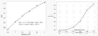
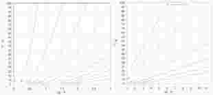
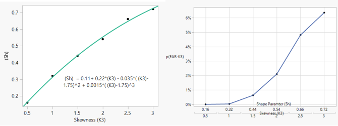
, which is delineated by two parameters, namely, the shape (Sh) or mean (µ) and the scale parameter (Sc) or standard deviation (σ). The FAR caused by skewness in a data distribution with control limits placed at ± 3 (σR) from the mean can be determined by knowing the relationship between the skewness value and shape parameter (Sh). A correlation expression between skewness and shape parameter (Sh) was developed from the data reported by Derya et al. (2012), as shown in Figure 4A
[12]
Karagöz, D., & Hamurkaroğlu, C. (2012). Control charts for skewed distributions: Weibull, gamma, and lognormal. Metodološki Zvezki, 9(2), 95–106.
. Using a scale parameter (Sc) = 0 and the shape parameter (Sh) calculated via the correlation shown in Figure 4A, the FAR for various degrees of skewness can be calculated via Equation (7), as shown in Figure 4B. Here, k is the number of standard deviations from the mean; for control limits placed at 3 SDs from the mean, k = 3. Figure 4B shows that a skewness below 1.5 keeps the control limit signal at an acceptable FAR of <1.0%.
Figure 4. (A) Correlation between skewness and log-normal shape factor. (B) FAR for an OOC signal from an asymmetric data distribution.
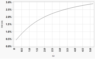
5.2. Modeling FAR for a Heavy-Tailed Distribution
Kurtosis is a measure of whether data are heavy-tailed or light-tailed relative to a normal distribution. Data distribution with high kurtosis tends to have heavy tails or outliers. In contrast, data distribution with low kurtosis tends to have light tails or a lack of outliers. A standard normal distribution has a kurtosis of zero. The kurtosis (K4) can be calculated from expression (8)
[11]
Richard A. Groeneveld, Glen Meeden, (1984). Measuring Skewness and Kurtosis, Journal of the Royal Statistical Society, 33(4), 391–399,
Braden, P., & Matis, T. (2022). Cornish–fisher-based control charts inclusive of skewness and kurtosis measures for monitoring the mean of a process. Symmetry, 14(6), 1176.
. A positive kurtosis indicates a "heavy-tailed" distribution. A t-distribution has fatter tails than a normal distribution. Therefore, a t-distribution can be used as a model to represent kurtosis, which will allow for a more realistic calculation of the FAR from excess kurtosis
[11]
Richard A. Groeneveld, Glen Meeden, (1984). Measuring Skewness and Kurtosis, Journal of the Royal Statistical Society, 33(4), 391–399,
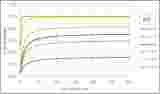
. The FAR caused by kurtosis can be modeled via a t-distribution, as expressed in (9) and as shown in Figure 5, by knowing the relationship between kurtosis (K4) and degrees of freedom (df) for the t-distribution. Here, k is the number of standard deviations from the mean; for control chart limits placed at 3 SDs from the mean, k = 3. dft.dist is the number of degrees of freedom for the t-distribution, and dft.dist can be calculated from the kurtosis (K4) in the data distribution, as expressed in (10)
[15]
Kenneth L. Lange, Roderick J. A. Little & Jeremy M. G. Taylor (1989) Robust Statistical Modeling Using the t Distribution, Journal of the American Statistical Association, 84(408), 881-896.
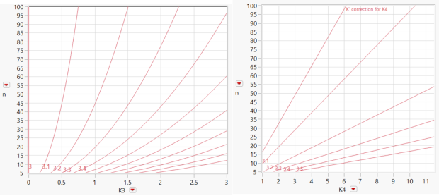
5.3. Adjustment to k to Accommodate Skewed and Heavy-Tailed Distributions
Braden et al. (2022) showed that the FAR for a severely skewed or heavy-tailed distribution can be reduced by replacing the control limits at k = 3 (σR) from the mean with limits based on adjusted k values (k’), as expressed in (11) and (12), to accommodate skewness or heavy tails in the data distribution. Branden also stated that Equations (11) and (12) are valid only when the skewness or kurtosis of the distribution meets the criteria expressed in (13)
[14]
Braden, P., & Matis, T. (2022). Cornish–fisher-based control charts inclusive of skewness and kurtosis measures for monitoring the mean of a process. Symmetry, 14(6), 1176.
Figure 6. (Left) Adjustment of k for skewness. (Right). Adjustment of k for kurtosis.
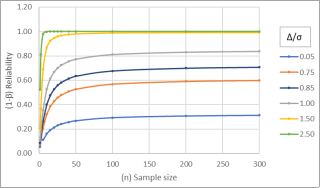
6. Nuisance Signal from Nelson Rule 2 and Its Reliability
According to Nelson rule 2, nine consecutive data points on one side of the center line can be used to detect a shift in the mean, which can result in a nuisance signal, as the magnitude of this shift in the mean can be potentially insignificant. Therefore, when a signal is identified for Nelson rule 2, it is imperative that the strength of the signal be assessed against the magnitude of the shift. Wheeler (2010) classified Nelson test rule 2 signals as small shift when magnitude of signal is less than 1.5 standard deviation from mean (Δ/σ). An intermediate shift when signal is 1.5 ≥ (Δ/σ) ≤ 2.5, and as a large shift when the magnitude of signal (Δ/σ) > 2.5
[16]
D J. Wheeler and R Stauffer. (2017). When Should We Use Extra Detection Rules? Using process behavior charts effectively. Quality Digest, 322, 1-14.
. The reliability of the signal for the desired shift effect can be calculated from the type II error. In control charts, the (β) value or type II error indicates the probability of a true signal going undetected. The widely acceptable minimum probability for β is 0.20
[17]
Muralidharan, N. (2023). Process Validation: Calculating the Necessary Number of Process Performance Qualification Runs. Bio-process International, 21(5), 37-43. https://bioprocessintl.com/analytical/upstream-validation/process-validation-calculating-the-necessary-number-of-process-performance-qualification-runs/
[17]
, which indicates a reliability (1–β) of 100% – 20% = 80%. The relationship between sample size, type I error (α), type II error (β), and shift from mean (Δ/σ) is expressed for two-sided limit and one-sided limit, as shown in (14) and (15)
[21]
NIST/SEMATECH. Engineering Statistics Handbook. National Institute of Standards and Technology: Gaithersburg, MD, 2012.
Here, nT is the total sample size in the analysis, where nT = nhis + nsis. nhis is the number of historic samples, and nSis is the number of data points on one side of the center line showing a positive signal for Nelson test rule 2: therefore, nSis = 9. df = nsig + nhis – 2, which represents the degrees of freedom, and t(1-α, df) represents the inverse of the cumulative t-distribution at 1 – α and df.
Here, an acceptable value of the significance (α) value or type I error is often set at 0.05
[18]
Kim H. Y. (2015). Statistical notes for clinical researchers: Type I and type II errors in statistical decision. Restorative dentistry & endodontics, 40(3), 249–252.
, indicating a 5% probability of falsely identifying a signal as positive when the data corresponds to normal variability within the process. In this case, the statistical confidence (1 – α) is 100% – 5% = 95%.
The detectability/shift from the mean (Δ/σ) is the acceptable distance from the mean, expressed as a number of standard deviations. The FDA guidance document on “statistical review and evaluation” states that a (Δ/σ) value of 1.5 at 95% confidence (1 – α) is adequate to conclude equivalence between two groups
[19]
Durivage M. (2016). How To Establish Sample Sizes for Process Validation Using Statistical Tolerance Intervals. Bioprocess Online
Equations (14) and (15) for the sample size are rearranged to solve for reliability (1-β) as expressed in (16) and (17), respectively. According to Cohen (1988), minimum reliability (1 – β) ≥ 80% is generally accepted to statistically conclude that no true signal is going un-noticed
[17]
Muralidharan, N. (2023). Process Validation: Calculating the Necessary Number of Process Performance Qualification Runs. Bio-process International, 21(5), 37-43. https://bioprocessintl.com/analytical/upstream-validation/process-validation-calculating-the-necessary-number-of-process-performance-qualification-runs/
[17]
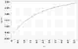
. Figure 7 shows the reliability of a signal for Nelson rule 2 for different combinations of the shift from the mean (Δ/σ) and historic sample size (nhis). Assuming signal sample size (nsig = 9; i.e. nine data points on one side of the center line for the Nelson test rule 2), the reliability is calculated via Equation (16) for different values of the shift from the mean (Δ/σ) as shown in Figure 7. Figure 7 demonstrates that if the observed shift in the mean is ≤1 SD, then the signal can be considered as a nuisance signal as the minimum reliability criteria of (1-β) ≥ 0.80 is not met even when the historical sample size nhis is as large as 100.
Figure 7. Reliability vs. sample size for different values of Δ/σ.
7. Conclusions
Challenges in CPV review sessions include assessing a control chart signal for reliability and deciding whether to initiate an investigation followed by action for a corrective or preventive action. However, control charts are susceptible to false alarms and nuisance alarms. Trusting incorrect signals from the control chart and initiating quality control actions can lead to a waste of resources and time. Therefore, it is imperative to understand false alarm probabilities in control charts in association with different Nelson test rules. In this article, we reviewed the current state of understanding on FARs inherent to control charts and the impact on FARs of data distributions that deviate from normal distribution assumptions. We also discussed methods for optimizing the use of control charts by selecting the Nelson test rules to be applied and correcting the number of sigma factors (k) used for calculating control limits to accommodate skewness and kurtosis in a data distribution to reduce the FAR and nuisance signals and to improve the reliability of data trending and monitoring.
Biologics manufacturing is complex and sometimes demands simultaneous monitoring of two or more related variables for improved understanding of process control to ensure product quality
[22]
Muralidharan, N., Johnson, T., & Davis, M. (2023). Identifying False Metabolite Measurements During Cell-Culture Monitoring Effective Application of the Multivariate Hotelling’s T2 Statistic. Bioprocess International, 21(11-12), 29-31.
In such instances, multivariate control chart based on the Hotelling T2 statistics method are frequently used. Future work will need to focus on false alarm rates inherent in multivariable control charts.
Abbreviations
df: Degrees of Freedom
FAR: False Alarm Rate
SD: Standard Deviation
OOC: Out-of-Control
Xbar: Sample Mean
p: Probability
nsig = 9: Number Samples on One Side of the Control Chart
nhis: Number of Samples Used for Historic Samples
K3: Kurtosis
K4: Skewness
k: Number of standard Deviations from the Mean for the Placement of Control Limits
Δ/σ: Number of Standard Deviations from the Mean for Considering the Reliability of a Shift in the Mean
β: Type II Error
α: Type I Error
µ: Population Mean
σ: Population Standard Deviation
Φ: Cumulative Normal Density Function
Author Contributions
Naveenganesh Muralidharan: Conceptualization, Writing – original draft, Review & editing
Thatsinee Johnson: Validation, Review
Leyla Saeednia Rose: Review
Mark Davis: Review
Disclaimer
The views and opinions expressed in this document are those of the authors only and do not necessarily reflect the official policy or position of AGC Biologics.
Conflicts of Interest
The authors declare no conflicts of interest.
References
[1]
Guidance for Industry: Process Validation — General Principles and Practices. US Food and Drug Administration: Silver Spring, MD, 2011;
Heigl, N., Schmelzer, B., Innerbichler, F., & Shivhare, M. (2021). Statistical quality and process control in Biopharmaceutical manufacturing—Practical issues and remedies. PDA Journal of Pharmaceutical Science and Technology, 75(5), 425-444.
Adams, B. M., Woodall, W. H., & Lowry, C. A. (1992). The use (and misuse) of false alarm probabilities in control chart design. Frontiers in Statistical Quality Control 4, 155-168.
Walker, E., Philpot, J. W., & Clement, J. (1991). False signal rates for the Shewhart control chart with supplementary runs tests. Journal of Quality Technology, 23(3), 247-252.
Griffiths, D., Bunder, M., Gulati, C., & Onizawa, T. (2010). The probability of an out of control signal from Nelson's supplementary zig-zag test. Journal of Statistical Theory and Practice, 4(4), 609-615.
Adhibhatta, S., DiMartino, M., Falcon, R., Haman, E., Legg, K., Payne, R., Pipkins, K., & Zamamiri, A. (2017). Continued process verification (CPV) signal responses in Biopharma. ISPE | International Society for Pharmaceutical Engineering.
Trietsch, D., & Bishak, D. (2007). The Rate of False Signals for Control Charts with Limits Estimated from Small Samples. Journal of Quality Technology, 39(1), 52-63.
Bischak, D. P., & Trietsch, D. (2007). The rate of false signals in u control charts with estimated limits. Journal of Quality Technology, 39(1), 54-65.
Munoz, J., Moya Fernandez, P., Alvarez, E., & Blanco-Encomienda, F. (2020). An alternative expression for the constant c4[n] with desirable properties. Scientia Iranica, 0(0), 3388-3393.
Braden, P., & Matis, T. (2022). Cornish–fisher-based control charts inclusive of skewness and kurtosis measures for monitoring the mean of a process. Symmetry, 14(6), 1176.
Kenneth L. Lange, Roderick J. A. Little & Jeremy M. G. Taylor (1989) Robust Statistical Modeling Using the t Distribution, Journal of the American Statistical Association, 84(408), 881-896.
Muralidharan, N. (2023). Process Validation: Calculating the Necessary Number of Process Performance Qualification Runs. Bio-process International, 21(5), 37-43. https://bioprocessintl.com/analytical/upstream-validation/process-validation-calculating-the-necessary-number-of-process-performance-qualification-runs/
[18]
Kim H. Y. (2015). Statistical notes for clinical researchers: Type I and type II errors in statistical decision. Restorative dentistry & endodontics, 40(3), 249–252.
Muralidharan, N., Johnson, T., Rose, L. S., Davis, M. (2024). CPV Monitoring - Optimization of Control Chart Design by Reducing the False Alarm Rate and Nuisance Signal. Science Journal of Applied Mathematics and Statistics, 12(2), 20-28. https://doi.org/10.11648/j.sjams.20241202.11
Muralidharan, N.; Johnson, T.; Rose, L. S.; Davis, M. CPV Monitoring - Optimization of Control Chart Design by Reducing the False Alarm Rate and Nuisance Signal. Sci. J. Appl. Math. Stat.2024, 12(2), 20-28. doi: 10.11648/j.sjams.20241202.11
Muralidharan N, Johnson T, Rose LS, Davis M. CPV Monitoring - Optimization of Control Chart Design by Reducing the False Alarm Rate and Nuisance Signal. Sci J Appl Math Stat. 2024;12(2):20-28. doi: 10.11648/j.sjams.20241202.11
@article{10.11648/j.sjams.20241202.11,
  author = {Naveenganesh Muralidharan and Thatsinee Johnson and Leyla Saeednia Rose and Mark Davis},
  title = {CPV Monitoring - Optimization of Control Chart Design by Reducing the False Alarm Rate and Nuisance Signal},
  journal = {Science Journal of Applied Mathematics and Statistics},
  volume = {12},
  number = {2},
  pages = {20-28},
  doi = {10.11648/j.sjams.20241202.11},
  url = {https://doi.org/10.11648/j.sjams.20241202.11},
  eprint = {https://article.sciencepublishinggroup.com/pdf/10.11648.j.sjams.20241202.11},
  abstract = {The Food and Drug Administration’s 2011 Process Validation Guidance and International Council for Harmonization Quality Guidelines recommend continued process verification (CPV) as a mandatory requirement for pharmaceutical, biopharmaceutical, and other regulated industries. As a part of product life cycle management, after process characterization in stage 1 and process qualification and validation in stage-2, CPV is performed as stage-3 validation during commercial manufacturing. CPV ensures that the process continues to remain within a validated state. CPV requires the collection and analysis of data related to critical quality attributes, critical material attributes, and critical process parameters on a minimum basis. Data is then used to elucidate process control regarding the capability to meet predefined specifications and stability via statistical process control (SPC) tools. In SPC, the control charts and Nelson rules are commonly used throughout the industry to monitor and trend data to ensure that a process remains in control. However, basic control charts are susceptible to false alarms and nuisance alarms. Therefore, it is imperative to understand the assumptions behind control charts and the inherent false alarm rates for different Nelson rules. In this article, the authors have detailed the assumptions behind the usage of control charts, the rate of false alarms for different Nelson rules, the impact of skewness and kurtosis of a data distribution on the false alarm rate, and methods for optimizing control chart design by reducing false alarm rates and nuisance signals.},
 year = {2024}
}
TY  - JOUR
T1  - CPV Monitoring - Optimization of Control Chart Design by Reducing the False Alarm Rate and Nuisance Signal
AU  - Naveenganesh Muralidharan
AU  - Thatsinee Johnson
AU  - Leyla Saeednia Rose
AU  - Mark Davis
Y1  - 2024/04/02
PY  - 2024
N1  - https://doi.org/10.11648/j.sjams.20241202.11
DO  - 10.11648/j.sjams.20241202.11
T2  - Science Journal of Applied Mathematics and Statistics
JF  - Science Journal of Applied Mathematics and Statistics
JO  - Science Journal of Applied Mathematics and Statistics
SP  - 20
EP  - 28
PB  - Science Publishing Group
SN  - 2376-9513
UR  - https://doi.org/10.11648/j.sjams.20241202.11
AB  - The Food and Drug Administration’s 2011 Process Validation Guidance and International Council for Harmonization Quality Guidelines recommend continued process verification (CPV) as a mandatory requirement for pharmaceutical, biopharmaceutical, and other regulated industries. As a part of product life cycle management, after process characterization in stage 1 and process qualification and validation in stage-2, CPV is performed as stage-3 validation during commercial manufacturing. CPV ensures that the process continues to remain within a validated state. CPV requires the collection and analysis of data related to critical quality attributes, critical material attributes, and critical process parameters on a minimum basis. Data is then used to elucidate process control regarding the capability to meet predefined specifications and stability via statistical process control (SPC) tools. In SPC, the control charts and Nelson rules are commonly used throughout the industry to monitor and trend data to ensure that a process remains in control. However, basic control charts are susceptible to false alarms and nuisance alarms. Therefore, it is imperative to understand the assumptions behind control charts and the inherent false alarm rates for different Nelson rules. In this article, the authors have detailed the assumptions behind the usage of control charts, the rate of false alarms for different Nelson rules, the impact of skewness and kurtosis of a data distribution on the false alarm rate, and methods for optimizing control chart design by reducing false alarm rates and nuisance signals.
VL  - 12
IS  - 2
ER  -