The main challenge of the well-celebrated Levenberg-Marquardt algorithm (LMA) is the selection of the searching direction and adaptation parameters. Secondly, the implementation of the LMA for online model identification has faced challenges as it is a batch optimization. As a third challenge, the solution of the Levenberg-Marquardt based on the full-Newton nonlinear optimization (FNNO) for online applications have been limited due to its unguaranteed positive definiteness. This paper presents two versions of the modified Levenberg-Marquardt algorithm (MLMA) for neural network model identification and adaptive predictive control for the online dynamic model identification and adaptive control of a self-balancing two-wheel LEGO Mindstorms NXTway-GS robot. The first version is the online-window-approach of the modified Levenberg-Marquardt algorithm (OWA-MLMA) based on approximate Guass-Newton algorithm (AGNA) for training neural network model predictor. The second version is a neural network-based adaptive predictive control (APC) algorithm based on the full-Newton nonlinear optimization of the modified Levenberg-Marquardt algorithm (FNNO-MLMA) for online adaptive control. A NNARMAX model predictor for the NXT robot is first trained and validated using the OWA-MLMA based on AGNA. The validated NNRAMAX model is then used for the design of the NN-APC based on FNNO-MLMA. Finally, the model identification based on OWA-MLMA and APC based on FNNO-MLMA schemes are simulated in closed-loop for online NNARMAX model identification and adaptive predictive control of the NXT robot. The comparison of the proposed OWA-MLMA based on AGNA shows superior performance over the recursive incremental back-propagation algorithm (INCBPA) while the proposed NN-APC based on FNNO-MLMA shows excellent control and good tracking performances over a discrete-time fixed-parameter proportional-integral-derivative (PID) controller for the NXT robot control. The simulation results show that the developed OWA-MLMA based on AGNA and the APC based on FNNO-MLMA can be adapted for the online dynamic modeling, automation, control and robotics applications.
| Published in | Automation, Control and Intelligent Systems (Volume 13, Issue 3) |
| DOI | 10.11648/j.acis.20251303.14 |
| Page(s) | 86-115 |
| Creative Commons |
This is an Open Access article, distributed under the terms of the Creative Commons Attribution 4.0 International License (http://creativecommons.org/licenses/by/4.0/), which permits unrestricted use, distribution and reproduction in any medium or format, provided the original work is properly cited. |
| Copyright |
Copyright © The Author(s), 2025. Published by Science Publishing Group |
Approximate Gauss Newton Algorithm (AGNA), Full-Newton Nonlinear Optimization (FNNO), LEGO Mindstorms NXT Robot, Modified Levenberg-Marquardt Algorithm (MLMA), Neural Networks, Nonlinear Adaptive Predictive Control (NAPC), Online-Window-Approach (OWA), Self-Balancing Two-Wheel Robot
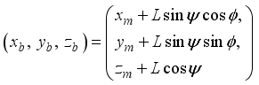
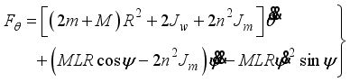
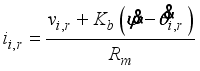
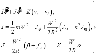
 is the body pitch angle,
  is the wheel angle (where l and r indicates left and right angles), and
  is the DC motor angle. The physical parameters of the NXT robot are defined in Table 1.
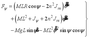
 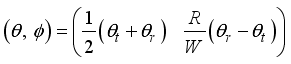 (1)
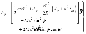
(1)  (2)
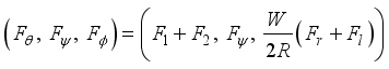
(2)  (3)
(3) S/N | Physical Parameters | Values | Units |
|---|---|---|---|
1 | Gravitational acceleration (g) | 9.810 | m.sec-2 |
2 | Wheel weight (m) | 0.030 | kg |
3 | Wheel radius (R) | 0.040 | m |
4 | Wheel inertia moment (JW) | mR2/2 | kg.m2 |
5 | Body weight (M) | 0.600 | kg |
6 | Body width (W) | 0.140 | m |
7 | Body depth (D) | 0.040 | m |
8 | Body height (H) | 0.144 | m |
9 | Distance of the centre of mass from the wheel axle (L) | H/2 | m |
10 | Body pitch inertia moment (Jψ) | ML2/3 | kg.m2 |
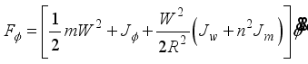
11 | Body yaw inertia moment (Jϕ) | M (W2 + D2)/12 | kg.m2 |
12 | DC motor inertia moment (Jm) | 1 x 10⁻⁵ | kg.m2 |
13 | DC motor resistance (Rm) | 6.690 | Ω |
14 | DC motor back EMF constant (Kb) | 0.468 | V.sec.rad-1 |
15 | DC motor torque constant (Kt) | 0.317 | Mn.A-1 |
16 | Gear ratio (n) | 1.000 | - |
17 | Friction coefficient between body and DC motor (fm) | 0.002 | - |
18 | Friction coefficient between wheel and floor (fW) | 0.000 | - |
 (4)
(4)  (5)
(5)  (6)
(6)  (7)
(7)  (8)
(8)  (9)
(9)  (10)
(10)  (11)
(11)  (12)
(12)  (13)
(13)  (14)
(14)  (15)
(15)  (16)
(16)  (17)
(17)  (18)
(18)  (19)
(19)  (20)
(20)  (21)
(21)  (22)
(22)  (23)
(23)  (24)
(24)  and
and  (25)
(25)  and neglect the second-order term like
  . The motion equations (13-15) are approximated according to the following equations respectively:
  (26)
(26)  (27)
(27)  (28)
(28)  (29)
(29) 
 (30)
(30)  (31)
(31)  (32)
(32)  (33)
(33)  (34)
(34)  (35)
(35)  (36)
(36) 
 and the body pitch angular velocity
  . It is easy to evaluate
  and
and  by using
  . There are two methods to evaluate
  by using
  , namely: 1). Derive
  by integrating the angular speed numerically and 2). Estimate
  by using an observer based on modern control theory. In this study, we use the second method in the following for the controller design chiefly because of easy stability establishment.
  of a discrete-time nonlinear m-input n-output multivariable system at time instant k responding to the lth input
  can be described by the following Nonlinear AutoRegressive Moving Average with eXogeneous input (NARMAX) model:
 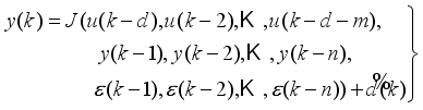 (37)
(37)  is a nonlinear function of its input arguments assumed to be differentiable,
 ,
, 
 and
and 
 are the vectors of the past input, past output and past prediction error values respectively while
  are the disturbances and d is the system delay. Assuming that the input-output data pair
  of the system taken over NT period of time is available
  (38)
(38)  (39)
(39)  is a known vector of appropriate dimension that defines the parameters of the system and
 is the state (regression) vector at time
  .
.  ,
,  , with an initial small random value of
  ; at time
  we can construct a predictor
  that will produce the a priori predictor estimate of (39)
  based on the state of the system
  at time
  can be define as
 is an unknown adjustable parameter vector of appropriate dimension and the regression (state) vector

 . Thus, at time
  a new value of
  will be known and the a posteriori predictor estimate can be computed as
  (40)
(40)  is compared to the system output
  and the error
  between the two outputs is minimized and used to adjust and update
  such that
  . It is evident that the predictor output depends on
  . For notational convenience, we define the error here as:
  (41)
(41)  ,
,  and
and  are the true system output, network predicted output and the adjustable parameters of the network. Thus, the determination and adjustment of
  becomes an unconstrained nonlinear minimization problem defined here as:
  (42)
(42)  is the value of
  that minimizes (42) and
  is formulated as a total square error (TSE) type cost function given as:
 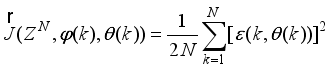 (43)
(43)  which is obtained from
  defined in (38).
  in (42) is decomposed into the past input, past output and past prediction error parts
  ,
, 
 and
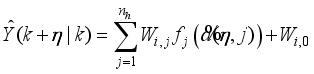
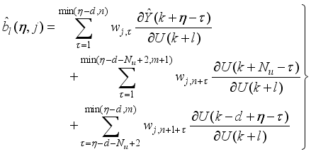
and  respectively. The outputs of the NN model of Figure 10 can be expressed in terms of the network parameters as:
 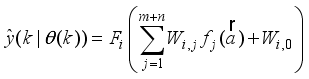 (44)
(44) 
 and
and  and
and  are the hidden and output weights respectively;
  and
and  are the hidden and output biases;
  is a linear activation function for the output layer and
  is an hyperbolic tangent activation function for the hidden layer given here as:
  (45)
(45)  .
. 
 ; where
  ,
,  is an identity matrix,
  and
and  are the weight decay values for the input-to-hidden and hidden-to-output layers respectively. Using (44), the regularized criterion from (43) becomes:
 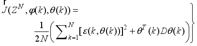 (46)
(46)  (47)
(47)  can be presented to the training algorithm at each time step. The most popular way being the batch (off-line) mode where all the data set
  is evaluated at each time step and the recursive (online) mode where each data pair of
  is evaluated at each time step.
  at each sampling time step and all the data are evaluated in batch mode at each sampling time step.
  and updates
  iteratively according to the following typical updating rule:
  (48)
(48)  denotes
  at the current iteration
 is the searching direction,
  is the global minimum and
  if certain stopping criteria are satisfied.
  is the back-propagation algorithm (BPA)
  directly proportional to the negative of the gradient of (46) evaluated at
  . Using (46) and (48), the basic BP algorithm can be stated as:
  (49)
(49)  is the step size and
  is the gradient NN training using the BPA has been reported to be characterized by poor performance
  (50)
(50)  given as
  (51)
(51)  from now on shall be used for convenience. Note that Equation (17) can also be expressed as
  (52)
(52)  (53)
(53)  (54)
(54)  and
and  are the gradient and exact Gauss-Newton Hessian matrices respectively, and
 denotes the derivative of the network output with respect to
  evaluated at
  . By substituting
  into (52) and setting its derivative to zero as follows:
 (55)
(55)  (56)
(56)  . Equation (54) is guaranteed to be positive definite since it is based a second-order approximation of (47) which is well-known to be positive definite
  especially when
  is far from
  and (53) can sometimes be ill-conditioned. In the next sub-section, we utilize (56) to formulate the proposed OWA-MLMA based on AGNA which addresses the above issues dynamically.
  to the diagonal of
  with a new updating rule given as
  (57)
(57)  (58)
(58)  characterizes a hybrid of searching directions and has several effects
  , Equation (57) reduces to the steepest descent algorithm (with step
  which requires a descend search method; and 2). for small values of
  , Equation (57) reduces to Gauss-Newton algorithm (with step given by (56)).
  is large
  , so that (58) becomes
  (59)
(59)  is adjusted simultaneously with
  in the search for
  by (57), s is the scaling parameter, and I is an identity. The solution to (57) using (59) based on the trust region method
  (60)
(60)  .
.  is the trust region radius within which
  can be found. A difficulty with the Levenberg-Marquardt method is in selecting and adjusting the parameter
  as well as how
  should be updated. The choice for the proper selection of
  has led to the formulation of several algorithms
  is adjusted based on the ratio
  between the actual reduction
  and theoretical predicted decrease
  subject to the constraint in (60) stated here as:
 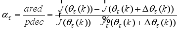 (61)
(61)  in (46) for convenience.
  D,
D,  and m and n for
  .
.  in (61).
  according to the following conditions on
  :
:  , then
  and go to Step6).
  , then
  and go to Step 6).
  and
and  .
.  or
or  or
or  (number of iterations); go to Step 8), else go to Step 3).
  and terminate.
  (62)
(62)  is the step size and
  is an identity matrix of appropriate dimension. Next, the basic back-propagation given as
 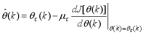 (63)
(63) 


 ,
,  and
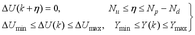
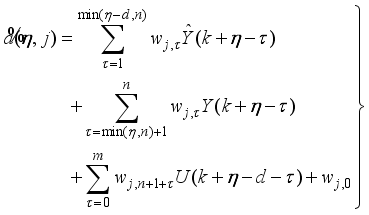
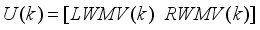
and  are the desired reference signal, prediction error, control input, system output, η step-delay prediction model output, η step-ahead predicted output, noise/input disturbances and ηstep-delay operator respectively and k is the number of samples based on the new measurement data sample.
 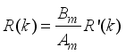 (64)
(64)  and
and  are the desired reference and the filtered reference signals respectively; Am and Bm are the denominator and numerator polynomials of the filter. In this way, the NAPC based on FNNO-MLMA is deigned, in part, based on the filter tracking error capability; where Am and Bm serves as tuning parameters used to improve the robustness and internal stability of the control algorithm respectively.
  at that same sample time instant k.
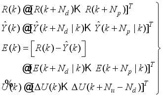
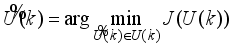
  , the NAPC based on FNNO-MLMA calculates a sequence of control inputs
  consisting of the current
  and future inputs
  . The current input
  is held constant after
  control moves; where
  is the maximum control horizon. The input
  is calculated such that a set of
  approaches the desired reference signal in an optimal manner over a specified prediction horizon
 where
where  and
and  are the minimum and maximum prediction horizons respectively.
  (65)
(65)  (66)
(66)  (67)
(67)  is the change in control signal;
  and
and  are two weighting matrices penalizing changes on
  and
and  in Equation (65).
  and NN model
  approximates the system (37),
  and that the system information is available up to time
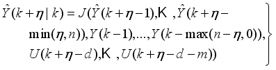
  , so that the one step-ahead predictor of (37) at time
  can be expressed as:
 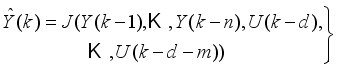 (68)
(68)  (69)
(69)  (70)
(70)  (71)
(71)  (72)
(72) 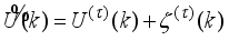 (73)
(73)  ; where
  is the current iterate of the control sequence; and
  the search direction given by the following expression:
 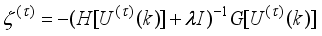 (74)
(74)  is the adaptation parameter, I is a diagonal matrix;
  and
and  are the Hessian and Jacobian matrices given respectively by (75) and (76) as follows:
 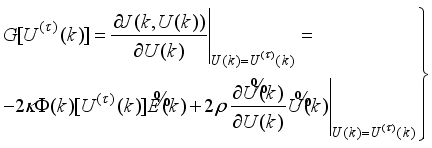 (75)
(75)  (76)
(76)  in (75), the control signal is decomposed into the past and future control signals as
  given in (77) as follows:
 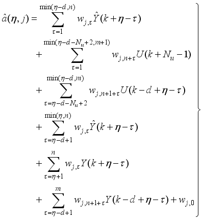 (77)
(77)  . Thus,
  is computed here based only on the future control signals
  and
and  as:
as: 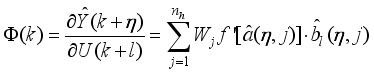
 (78)
(78)  for all
  , and for all
  is calculated as follows:
 (79)
(79)  ,
,  ,
, 
 (80)
(80) Initialize: for while for for
if for
end for b, end for a if for
end for a else for
for
end for b, end for a, end for a, end if La,a, end for kn
if end while |
 that will satisfy this condition. Again, many algorithms have been proposed for this purpose
  and re-computes (80) and then terminates immediately positive definite of (80) is achieved.
  (81)
(81)  (82)
(82)  is the trust region radius where
  can be trusted.
  in (81) is to be updated and the step size at the next iteration. Although, many algorithms have been proposed for this purpose
  obtained from Table 2 for this purpose. Note that
  characterizes a hybrid adaptation parameter and has several effects as discussed in Section 3.1.3. Unlike in Section 3.1.3 where the approximated
  is guaranteed to be positive definite, here
  is not guaranteed to be non-positive definite or ill-conditioned and the algorithm of Table 2 is used.
  obtained in Table 2 and apply the indirect method discussed in Section 3.1.4 to
  is adjusted according to the ratio
  between the actual reduction
  and theoretical predicted decrease
  as defined below:
  (83)
(83)  and evaluate
  using (65) subject to (66). Initialize
  ,
,  and set
  . while
  .
.  using (77).
  according to the conditions on
  :
:  , then
  and go to Step 7).
  , then
  and go to Step 7).
  update
  and set
  .
.  is defined as follows:
 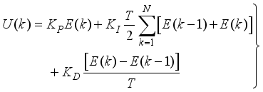 (84)
(84)  and
and  are the proportional, integral and derivative gains respectively,
  is the sampling time and
 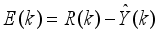 is the error term defined as the difference between the process
  , filtered desired reference
  and N is the number of simulation samples (see sub-section 4.1.1).
  is selected as the reference signal for servo control. It is important to note that we cannot use variables other than
  as the reference because the system may become uncontrollable. The block diagram of the preliminary servo controller for NXTway-GS robot is shown in Figure 13.
 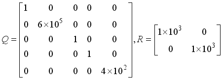 (85)
(85)  ,
,  and
and  are the tuning parameters.
  (86)
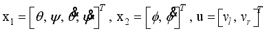
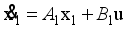
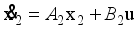
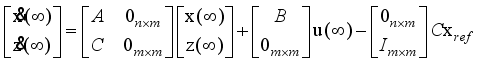
(86)  , an integral of the difference
  , states of the expansion system
  , and the orders of x and u are n and m respectively. The state equation of the expansion system is the following:
  (87)
(87)  (88)
(88) 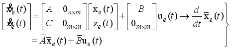 (89)
(89)  ,
,  and
and  . We can use feedback control to make the expansion system stable. Thus, the control input is becomes
  (90)
(90)  ,
,  and
and  are assumed, the following input
  can be derived as:
  (91)
(91)  . The input vector
  to the NNARMAX model predictor consists of the regression vectors
  ,
, 
 and
and 

 . The outputs of the NNARMAX model predictor are the predicted values of LWRA and RWRA given as
  .
.  ,
,  ,
,  ,
,  ,
,  ,
,  for the NNARMAX model predictors as well as
  ,
,  ,
,  and
and  . The details of these parameters are discussed in section 3; where
  and
and  are the number of inputs and outputs of the system,
  and
and  are the orders of the regressors,
  is the total number of regressors (that is, the total number of inputs to the network),
  and
and  are the number of hidden and output layers neurons, and
  and
and  are the hidden and output layers weight decay terms. Also,
  is selected to initialize the INCBPA while
  ,
,  and
and  are arbitrarily selected to initialize the OWA-MLMA. The network is trained for τ = 20 iterations with the just mentioned selected parameters.
 S/N | Performance Evaluation Parameters | Left wheel rotation angle | Right wheel rotation angle | ||
|---|---|---|---|---|---|
INCBPA | OWA-MLMA | INCBPA | OWA-MLMA | ||
1 | Computation time for model identification (sec) | 5.8120e+02 | 1.5109e+03 | 5.7036e+02 | 1.3225e+03 |
2 | Minimum performance index (MPI) | 5.2343e-02 | 4.4952e-05 | 2.6659e-02 | 8.0105e-05 |
3 | Total square error (TSE) | 4.1499e+01 | 9.5898e-03 | 1.1104e+01 | 2.6953e-03 |
4 | Mean error of one step ahead prediction of training data | 1.0442e-01 | 1.1104e-04 | 7.0847e-01 | 2.6953e-04 |
5 | Mean error of one step prediction of test data | 3.2832e+01 | 5.1594e-02 | 2.8006e+01 | 1.1955e-03 |
6 | Mean value of 5-step ahead prediction error | 4.8886e+01 | 5.0041e-02 | 5.1418e+01 | 5.0736e-02 |
7 | Akaike’s final prediction error (AFPE) estimate | 3.7989e+01 | 9.8119e-02 | 5.1532e+01 | 1.4494e-02 |
Constraint Parameters | Fixed-Parameter PID Controller | NAPC based on FNNO-MLMA | ||
|---|---|---|---|---|
LWRA | RWRA | LWRA | RWRA | |
Minimum control input (umin) | -10 | -10 | -10 | -10 |
Maximum control input (umax) | 10 | 10 | 10 | 10 |
Minimum predicted output (ymin) | -0.5 | -0.5 | -0.5 | -0.5 |
Maximum predicted output (ymax) | 10 | 10 | 10 | 10 |
Minimum desired reference (Refmin) | -100 | -100 | -100 | -100 |
Maximum desired reference (Refmax) | 100 | 100 | 100 | 100 |
Tuning Parameters | Fixed-Parameter PID Controller | NAPC based on FNNO-MLMA | ||
|---|---|---|---|---|
LWRA | RWRA | LWRA | RWRA | |
ICI (u) | -80 | -80 | -10 | -10 |
IPO (y) | 0 | 0 | 0 | 0 |
Nd | - | 1 | 1 | 1 |
Nu | - | 2 | 3 | 2 |
Np | - | 5 | 7 | 5 |
Κ | - | 1 | 1.5 | 1 |
ρ | - | 0.8 | 0.08 | 0.08 |
λ | - | - | 0.1 | 0.7 |
Am | [1-0.7] | [1-0.7] | [1-0.7] | [1-0.7] |
Bm | [00.3] | [00.3] | [00.3] | [00.3] |
Globmin | - | - | 7 | 5 |
δ | - | - | 1e-6 | 1e-4 |
uiter | - | - | 10 | 8 |
KP | 30 | - | - | - |
KI | 500 | - | - | - |
KD | 100 | - | - | - |
AFPE | Akaike’s Final Prediction Error |
AGNA | Approximate Gauss-Newton Algorithm |
BPA | Back-propagation Algorithm |
FNNO | Full-Newton Nonlinear Optimization |
INCBP | Incremental Back-propagation |
LMA | Levenberg-Marquardt Algorithm |
MLMA | Modified Levenberg-Marquardt Algorithm |
MBPC | Model-base Predictive Control |
MPI | Minimum Performance Index |
MRAC | Model Reference Adaptive Control |
NAPC | Nonlinear Adaptive Predictive Control |
NN | Neural Network |
NNARMAX | Neural Network Nonlinear Autoregressive Moving Average with Exogenous Input |
OWA | Open-window-approach |
PID | Proportional-integral-derivative |
TSE | Total Square Error |
| [1] | P. Corke, “Robotics, Vision and Control Fundamental Algorithms in MATLAB®,” 2nd Edition, Springer Springer-Verlag, Heidelberg, 2017. |
| [2] | P. H. Petkov, T. N. Slavov and J. K. Kralev “Design of Embedded Robust Control Systems Using MATLAB®/Simulink®,” The Institution of Engineering and Technology, London, United Kingdom, 2018. |
| [3] | C. S. Chin, “Computer-Aided Control System Design: Practical Applications Using MATLAB® and Simulink®,” CRC Press - Taylor & Francis Group, Raton, USA, 2013. |
| [4] | K. Ogata, “Modern Control Engineering,” Pearson Education, Inc., Prentice Hall, Upper Saddle River, New Jersey, USA, 2010. |
| [5] | W. S. Levine, “The Control Handbook: Control System Advanced Methods,” Second Edition, CRC Press - Taylor & Francis Group, New York, USA, 2011. |
| [6] | N. S. Nise, “Control Systems Engineering,” Seventh Edition, John Wiley & Sons Inc., California, USA. |
| [7] | A. A. Bobtsov, A. A. Pyrkin, S. A. Kolyubin, S. V. Shavetov, S. A. Chepinskiy, Y. A. Kapitanyuk, A. A. Kapitonov, V. M. Bardov, A. V. Titov and M. O. Surov, “Using of LEGO Mindstorms NXT Technology for Teaching of Basics of Adaptive Control Theory,” IFAC Proceedings Volumes, vol. 44, no. 1, pp. 9818-9823, 2011. |
| [8] | S. A. Fillippov, A. L. Fradkov, I. V. Ashikhmina and R. E. Seifullaev, “LEGO Mindstorms NXT Robot and Oscillators in Control Education,” IFAC Proceedings Volumes, vol. 43, no. 11, pp. 156-160, 2010. |
| [9] | B. A. Aleexeevich, A. K. Yuri, A. K. Alexander, A. K. Sergey, P. A. Alexandrovich, A. C. Sergey and V. S. Sergey, “LEGO Mindstorms NXT for Teaching the Principles of Adaptive Control to Students,” Sci. & Tech. J. of Inf. Tech., Mech. and Opt., vol. 355, no. 1(71), pp. 103-108, 2011. |
| [10] | M. Canale and S. Casale-Brunet, “A multidisciplinary approach for Model Predictive Control Education: A Lego Mindstorms NXT-based framework,” Int. J. of Cont., Aut. & Sys, vol. 12, no. 5, pp. 1030 - 1039, 2014. |
| [11] | H. L. Araujo, J. G. Agudelo, R. C. Vidal, J. A. Uribe, J. F. Remolina, C. Serpa-Imbett, A. M. López and D. P. Guevara, “Autonomous Mobile Robot Implemented in LEGO EV3 Integrated with Raspberry Pi to Use Android-Based Vision Control Algorithms for Human-Machine Interaction,” Mach., vol. 10 no. 193, pp. 1-20, 2022. |
| [12] | J. Y. Chen, T. F. Wu, P. S. Tsai and K. Y. Lian, “Indirect Adaptive Fuzzy Controller for LEGO Mindstorms NXT Two-Wheeled Robot,” App. Mech. & Mat., vols. 278-280, pp. 561-567, 2013, |
| [13] | H C. Ащепкова “Development of adaptive control system of model of the robot-loader on the basis of Lego Mindstorms NXT,” Tech. Aud. & Prod. Res., vol. vol. 5(6), no. 25, pp. 45-48, 2015. |
| [14] | A. Mitov, J. Kralev, T. Slavov and I. Angelov, “Comparison between Model Predictive (MPC) and Model Reference Adaptive Controllers (MRAC) for Electrohydraulic Steering System Implemented as Real-Time Simulink® Program,” IOP Conf. Series: Mat. Sci. and Eng., vol. 1002, no. 012034, pp. 1-12, 2020. |
| [15] | V. A. Akpan and G. D. Hassapis, “Training dynamic feedforward neural networks for online nonlinear model identification and control applications,” Int. Rev. of Aut. Cont.: Theo. & App., vol. 4, no. 3, pp. 335 - 350, 2011. |
| [16] | V. A. Akpan and G. D. Hassapis, “Nonlinear model identification and adaptive model predictive control using neural networks,” ISA Trans.; vol. 5, no. 2, pp. 177-94, 2011. |
| [17] |
V. A. Akpan, “Development of new model adaptive predictive control algorithms and their implementation on real-time embedded systems,” Aristotle university of Thessaloniki, GR-54124, Thessaloniki, Greece, Ph.D. Dissertation, 517 pages, July, 2011. Available:
http://invenio.lib.auth.gr/record/127274/files/GRI-2011-7292.pdf |
| [18] | L. Kalra and C. Georgakis, “Effects of process nonlinearity on the performance of linear model predictive controllers for the environmentally safe operation of a fluid catalytic cracking unit,” Ind. Eng. Chem. Res, vol. 33, pp.3063-3069, 1994. |
| [19] | S. J. Qin and T. A. Badgwell, “A survey of model predictive control technology,” Cont. Eng. Pract., vol. 11, pp. 733 - 764, 2003. |
| [20] | V. A. Akpan, I. K. Samaras and G. D. Hassapis, “Implementation of Network Control System over a Service-Oriented-Architecture Computer Network Based on Device Profile for Web Services for Industrial Control Applications,” Int. J. of Cont. Sci. & Eng., vol. 12, no. 1, pp. 1-25, 2022. Available: |
| [21] | N. Khaled and B. Pattel, “Practical Design and Application of Model Predictive Control: MPC for MATLAB® and Simulink® Users,” Butterworth-Heinemann, Oxford, United Kingdom, 2018. |
| [22] | L. Grüne and J. Pannek, “Nonlinear Model Predictive Control: Theory and Algorithms,” Second Edition, Springer International Publishing, Switzerland, 2017. |
| [23] | G. Colin, Y. Chamaillard, G. Bloch and G. Corde, “Neural control of fast nonlinear systems - Application to turbocharged SI engine with VCT,” IEEE Trans. Neu. Net., vol. 18, no. 4, pp. 1101 - 1114, Jul. 2007. |
| [24] | C. Lu and C. Tsai, “Adaptive predictive control with recurrent neural network for industrial process: An application to temperature control of a variable-frequency oil-cooling machine,” IEEE Trans. Ind. Elect., vol. 55, no. 3, pp. 1366-1375, Mar. 2008. |
| [25] | Y. Yamamoto, “NXTway-GS Model-Based Design: Control of self-balancing two-wheeled robot built with LEGO Mindstorms NXT,” Cybernet Systems Co. Limited, Revision 1.4, pp. 1 - 73, 2009. |
| [26] | The MathWorks Inc., MATLAB® & Simulink® 2025, Natick, USA. Available: |
| [27] | L. Lung, “System Identification: Theory for the User,” 2nd ed. Upper Saddle River, NJ: Prentice-Hall, 1999. |
| [28] | R. Chiong, “Intelligent Systems for Automated Learning and Application: Emerging Trends and Application,” Hershey PA, USA: Information Science Reference, 2010, ch. 4, pp. 204 - 316. |
| [29] | J. Wu, “Multilayer pottsperceptrons with Levenberg-Marquardt learning,” IEEE Trans. Neu. Net., vol. 19, no. 12, pp. 2032-2043, Dec. 2008. |
| [30] | V. A. Akpan and R. A. O. Osakwe, “Multivariable NNARMAX Model Identification of an AS-WWTP Using ARLS (Part 1: Dynamic Modeling of the Biological Reactors),” American J. of Int. Sys., vol. 4, no. 2, pp. 43 - 72, 2014. Available: |
| [31] | V. A. Akpan and R. A. O. Osakwe, “Multivariable NNARMAX Model Identification of an AS-WWTP Using ARLS (Part 2: Dynamic Modeling of the Secondary Settler and Clarifier),” American J. of Int. Sys., vol. 4, no. 3, pp. 77 - 106, 2014. Available: |
| [32] | V. A. Akpan and R. A. O. Osakwe, “Online Prediction of Influent Characteristics for Wastewater Treatment Plants Management Using Adaptive Recursive NNARMAX Model,” American J. of Int. Sys., vol. 4, no. 3, pp. 107 - 130, 2014. Available: |
| [33] | D. E. Rumelhart, G. E. Hinton and R. J. Williams, “Learning representations by back-propagating errors,” Nat., vol. 323, pp. 533-536, 1986. |
| [34] | P. J. Werbos, “Backpropagation through time: What it does and how to do it,” In Proc. IEEE, vol. 78, no. 10, pp. 1550 - 1560, Oct. 1990. |
| [35] | J. E. Dennis and R. B. Schnabel, “Numerical Methods for Unconstrained Optimization and Nonlinear Equations,” Englewood Cliffs, NJ: Prentice-Hall, 1996. |
| [36] | M. T. Hagan and M. B. Menhaj, “Training feedforward network with the Marquardt algorithm,” IEEE Trans. Neu. Net., vol. 5, no. 6, pp. 989-993, Nov. 1994. |
| [37] | R. Fletcher, “Practical Methods of Optimization,” 2nd ed., Chichester: Wiley & Sons, 1987. |
| [38] | K. Levenberg, “A method for the Solution of Certain Non-Linear,” Problems in Least Squares”, Quart. ofAppl Math., vol. 2, no. 2, pp. 164 - 168, 1944. |
| [39] | D. W. Marquardt, “An algorithm for least-squares estimation of nonlinear parameters,” J. Soc. for Ind. & Appl. Math., vol. 11, no. 2, pp. 431-441, 1963. |
| [40] | J. Hertz, A. Krough and R. G. Palmer, “An Introduction to the Theory of Neural Computation,” Lecture Notes, vol. 1, Redwood City, California: Addison-Wesley, 1991. |
| [41] | J. T. Spooner, M. Maggiore, R. Ordóñez and K. M. Passion, “Stable Adaptive Control and Estimation for Nonlinear Systems: Neural and Fuzzy Approximator Techniques,” New York: John Wiley & Sons, 2002. |
| [42] | O. M. Omidvar and D. L. Elliot, “Neural systems for control,” Academic Press, February, 1997. Available: |
| [43] | A. Visioli, “Practical PID Control,” London: Springer-Verlag Ltd., 2006. |
| [44] | L. Wang, S. Chai, D. Yoo, L. Gan and K. Ng, “PID and Predictive Control of Electrical Drives and Power Converters using MATLAB®/SIMULINK®,” IEEE John Wiley & Sons Singapore Pte. Ltd, 2015. |
| [45] | J. Sjöberg and L. Ljung, “Overtraining, regularization, and searching for minimum in neural networks,” Int. J. of Cont., vol. 62: 1391-1408, 1995. |
| [46] | The MathWorks Inc.., “Parallel Computing Toolbox™,” March, 2025. The MathWorks, Inc. 3 Apple Hill Drive, Natick, MA 0170-2098, USA. Available: |
| [47] |
V. A. Akpan, D. Chasapis and G. D. Hassapis, “FPGA Implementation of Neural Network-Based AGPC for Nonlinear F-16 Aircraft Auto-Pilot Control: Part 1 - Modeling, Synthesis, Verification and FPGA-in-the-Loop Co-Sim,” American J. of Emb. Sys. & Appl., vol. 9, no. 1, pp. 6-36 pages, 2022. Available:
https://www.sciencepg.com/journal/paperinfo?journalid=236&doi=10.11648/j.ajesa.20220901.13 |
| [48] | V. A. Akpan, D. Chasapis and G. D. Hassapis, “FPGA Implementation of Neural Network-Based AGPC for Nonlinear F-16 Aircraft Auto-Pilot Control: Part 2 - Implementation of Embedded PowerPC™440 with AGPC,” American J. of Emb. Sys. & Appl., vol. 9, no. 2, pp. 37-65, 2022. Available: |
APA Style
Akpan, V. A., Fatai, A., Ogidan, O. K. (2025). Neural Network-Based Online Model Identification and Nonlinear Adaptive Predictive Control of Self-Balancing Two-Wheel LEGO Mindstorms NXTway-GS Robot. Automation, Control and Intelligent Systems, 13(3), 86-115. https://doi.org/10.11648/j.acis.20251303.14
ACS Style
Akpan, V. A.; Fatai, A.; Ogidan, O. K. Neural Network-Based Online Model Identification and Nonlinear Adaptive Predictive Control of Self-Balancing Two-Wheel LEGO Mindstorms NXTway-GS Robot. Autom. Control Intell. Syst. 2025, 13(3), 86-115. doi: 10.11648/j.acis.20251303.14
@article{10.11648/j.acis.20251303.14,
  author = {Vincent Andrew Akpan and Ahmed-Ade Fatai and Olugbenga Kayode Ogidan},
  title = {Neural Network-Based Online Model Identification and Nonlinear Adaptive Predictive Control of Self-Balancing Two-Wheel LEGO Mindstorms NXTway-GS Robot
},
  journal = {Automation, Control and Intelligent Systems},
  volume = {13},
  number = {3},
  pages = {86-115},
  doi = {10.11648/j.acis.20251303.14},
  url = {https://doi.org/10.11648/j.acis.20251303.14},
  eprint = {https://article.sciencepublishinggroup.com/pdf/10.11648.j.acis.20251303.14},
  abstract = {The main challenge of the well-celebrated Levenberg-Marquardt algorithm (LMA) is the selection of the searching direction and adaptation parameters. Secondly, the implementation of the LMA for online model identification has faced challenges as it is a batch optimization. As a third challenge, the solution of the Levenberg-Marquardt based on the full-Newton nonlinear optimization (FNNO) for online applications have been limited due to its unguaranteed positive definiteness. This paper presents two versions of the modified Levenberg-Marquardt algorithm (MLMA) for neural network model identification and adaptive predictive control for the online dynamic model identification and adaptive control of a self-balancing two-wheel LEGO Mindstorms NXTway-GS robot. The first version is the online-window-approach of the modified Levenberg-Marquardt algorithm (OWA-MLMA) based on approximate Guass-Newton algorithm (AGNA) for training neural network model predictor. The second version is a neural network-based adaptive predictive control (APC) algorithm based on the full-Newton nonlinear optimization of the modified Levenberg-Marquardt algorithm (FNNO-MLMA) for online adaptive control. A NNARMAX model predictor for the NXT robot is first trained and validated using the OWA-MLMA based on AGNA. The validated NNRAMAX model is then used for the design of the NN-APC based on FNNO-MLMA. Finally, the model identification based on OWA-MLMA and APC based on FNNO-MLMA schemes are simulated in closed-loop for online NNARMAX model identification and adaptive predictive control of the NXT robot. The comparison of the proposed OWA-MLMA based on AGNA shows superior performance over the recursive incremental back-propagation algorithm (INCBPA) while the proposed NN-APC based on FNNO-MLMA shows excellent control and good tracking performances over a discrete-time fixed-parameter proportional-integral-derivative (PID) controller for the NXT robot control. The simulation results show that the developed OWA-MLMA based on AGNA and the APC based on FNNO-MLMA can be adapted for the online dynamic modeling, automation, control and robotics applications.
},
 year = {2025}
}
TY  - JOUR
T1  - Neural Network-Based Online Model Identification and Nonlinear Adaptive Predictive Control of Self-Balancing Two-Wheel LEGO Mindstorms NXTway-GS Robot

AU  - Vincent Andrew Akpan
AU  - Ahmed-Ade Fatai
AU  - Olugbenga Kayode Ogidan
Y1  - 2025/09/25
PY  - 2025
N1  - https://doi.org/10.11648/j.acis.20251303.14
DO  - 10.11648/j.acis.20251303.14
T2  - Automation, Control and Intelligent Systems
JF  - Automation, Control and Intelligent Systems
JO  - Automation, Control and Intelligent Systems
SP  - 86
EP  - 115
PB  - Science Publishing Group
SN  - 2328-5591
UR  - https://doi.org/10.11648/j.acis.20251303.14
AB  - The main challenge of the well-celebrated Levenberg-Marquardt algorithm (LMA) is the selection of the searching direction and adaptation parameters. Secondly, the implementation of the LMA for online model identification has faced challenges as it is a batch optimization. As a third challenge, the solution of the Levenberg-Marquardt based on the full-Newton nonlinear optimization (FNNO) for online applications have been limited due to its unguaranteed positive definiteness. This paper presents two versions of the modified Levenberg-Marquardt algorithm (MLMA) for neural network model identification and adaptive predictive control for the online dynamic model identification and adaptive control of a self-balancing two-wheel LEGO Mindstorms NXTway-GS robot. The first version is the online-window-approach of the modified Levenberg-Marquardt algorithm (OWA-MLMA) based on approximate Guass-Newton algorithm (AGNA) for training neural network model predictor. The second version is a neural network-based adaptive predictive control (APC) algorithm based on the full-Newton nonlinear optimization of the modified Levenberg-Marquardt algorithm (FNNO-MLMA) for online adaptive control. A NNARMAX model predictor for the NXT robot is first trained and validated using the OWA-MLMA based on AGNA. The validated NNRAMAX model is then used for the design of the NN-APC based on FNNO-MLMA. Finally, the model identification based on OWA-MLMA and APC based on FNNO-MLMA schemes are simulated in closed-loop for online NNARMAX model identification and adaptive predictive control of the NXT robot. The comparison of the proposed OWA-MLMA based on AGNA shows superior performance over the recursive incremental back-propagation algorithm (INCBPA) while the proposed NN-APC based on FNNO-MLMA shows excellent control and good tracking performances over a discrete-time fixed-parameter proportional-integral-derivative (PID) controller for the NXT robot control. The simulation results show that the developed OWA-MLMA based on AGNA and the APC based on FNNO-MLMA can be adapted for the online dynamic modeling, automation, control and robotics applications.

VL  - 13
IS  - 3
ER  -
Department of Biomedical Engineering, The Federal University of Technology, Akure, Nigeria
Biography: Vincent Andrew Akpan obtained his B. Sc. (Hons) degree in Physics from Delta State University, Abraka, Delta State, Nigeria in 1997; a Master of technology (M. Tech) degree in Electronic Measurement & Instrumentation from The Federal University of Technology, Akure, Ondo State, Nigeria in 2003; and a Ph.D degree in Electrical & Computer Engineering from Aristotle University of Thessaloniki, Thessaloniki, Greece in 2011. He is currently a Professor with the Department of Biomedical Engineering, School of Electrical Systems Engineering, The Federal University of Technology (FUTA), Akure, Nigeria. He was Head of the Department of Biomedical Technology, FUTA between 2017 and 2024. His research interest is in artificial intelligence, advanced electronic instrumentation, intelligent adaptive control, automation and embedded systems engineering. He is the co-author of a book and has authored and/or co-authored more than 90 articles in refereed journals and conference proceedings. He is a reviewer of several local and international journals as well as conference proceedings. Prof. Akpan was one among two Nigerian recipients of the 2005 Bilateral Education Agreement (BEA) scholarship tenable in Greece for a P.hD programme. He has won several research grants. Prof. Akpan is a member of several local and international professional societies.
Research Fields: artificial intelligence, automation, electronic instrumentation, industrial networked control systems, intelligent adaptive control systems, real-time embedded systems, robotics.

Department of Physics Electronics, The Federal University, Lokojae, Nigeria
Biography: Ahmed-Ade Fatai obtained his Higher National Diploma (HND) in Physics Electronics from The Federal Polytechnic, Idah, Kogi State, Nigeria in 2010; Postgraduate Diploma (PGD) in Physics Electronics from the Federal University of Technology, Akure, Odo State, Nigeria in 2013; and a Master of Technology (M. Tech.) degree in Electronic Measurement and Instrumentation from The Federal University of Technology, Akure, Nigeria in 2019. He is currently a Principal Technologist with the Department of Physics Electronics, The Federal University, Lokoja, Kogi State, Nigeria. He is currently working towards his Ph.D degree in Electronic Measurement and Instrumentation with The Department of Physics Electronics, The Federal University of Technology, Akure, Nigeria. His research interest is in instrumentation, intelligent adaptive control and embedded systems engineering. He has authored and co-authored more 7 articles in refereed journals and conference proceedings. Mr. Fatai is a member of the Nigeria Institute of Science Laboratory Technologist (NISLT).
Research Fields: electronic communication, electronic instrumentation, intelligent adaptive control, real-time embedded systems.

Department of Electrical and Electronics Engineering, Elizade University, Ilara-Mokin, Nigeria
Biography: Olugbenga Kayode Ogidan received a B. Eng (Hons) degree in Electrical and Electronics Engineering from the University of Ado Ekiti, Ekiti State, Nigeria in 2001; a Master of Electrical and Electronics Engineering degree from The Federal University of Technology, Akure, Ondo State, Nigeria in 2010; and Ph.D degree in Electrical Engineering from the Cape Peninsula University of Technology (CPUT), South Africa in 2015. He is currently an Associate Professor with the Department of Electrical and Electronics Engineering, Faculty of Engineering, Elizade University, Ilara-Mokin, Ondo State, Nigeria. His research interests include Smart Irrigation System, Internet of Things (IoT), Real-time systems, Networked Control Systems and Renewable Energy. He is currently the Acting Director, Entrepreneurship Development Centre, Elizade University, Ilara-Mokin, Ondo State, Nigeria. His research tagged “Solar Powered Smart Irrigation System” received first place award nationwide in the Nigerian Academy of Engineering Inaugural Innovation Challenge in 2024. Dr. Ogidan is a recipient of two national patent awards from the Federal Government of Nigeria. Dr. Ogidan is one of the two African scholars to receive the Climate Action Grant from the Association of Commonwealth Universities, UK in 2021. He is a registered member of the Council for the Regulation of Engineering in Nigeria (COREN) and the Computer Professional Registration Council of Nigeria (CPN).
Research Fields: electronic instrumentation, Internet of things (IoT), networked control systems, real-time systems, renewable systems, solar powered smart irrigation systems.

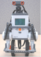
Figure 1. Self-balancing two-wheeled LEGO Mindstorms NXTway-GS.
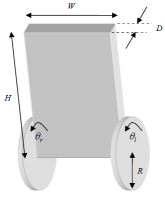
Figure 2. The schematic of the two-wheeled inverted pendulum robot.
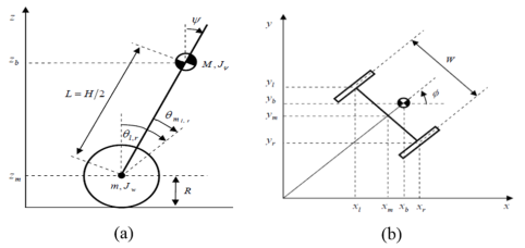
Figure 3. (a) Side view and (b) the plane view of the two-wheeled inverted pendulum.
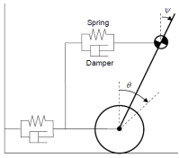
Figure 4. Equivalent mass-spring-damper system for one side of the two-wheeled inverted pendulum of the NXT robot.
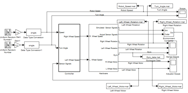
Figure 5. Simulink model of the self-balancing two-wheel NXT robot.
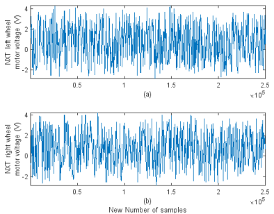
Figure 6. The NXT robot motor input voltage (V): (a) Left wheel motor and (b) Right wheel motor.
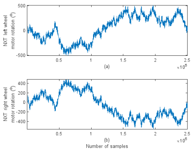
Figure 7. The NXT robot output wheel rotation in degrees (°): (a) Left wheel rotation and (b) Right wheel rotation.
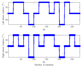
Figure 8. The desired reference trajectories for the NXT Robot.
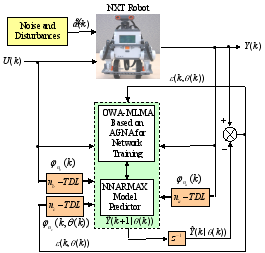
Figure 9. The NXT robot NNARMAX model identification scheme using OWA-MLMA training algorithm.
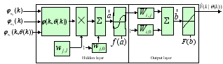
Figure 10. Architecture of the dynamic feedforward NN (DFNN) model.
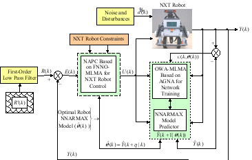
Figure 11. The NAPC-based FNNO-MLMA control scheme for the NXT robot control with the OWA-MLMA based on AGNA for training the NNARMAX model predictor.
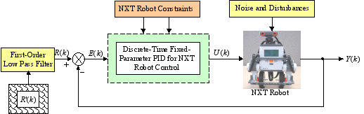
Figure 12. The discrete-time fixed-parameter PID control scheme.
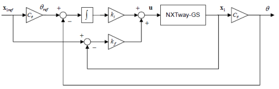
Figure 13. The Simulink® model of the NXT robot servo controller.
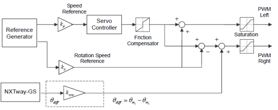
Figure 14. The complete Simulink® model of the NXT robot PID controller incorporating the servo controller of Figure 13. Note that the dashed block is a proportional controller for wheel synchronization when NXT robot doe not rotate.
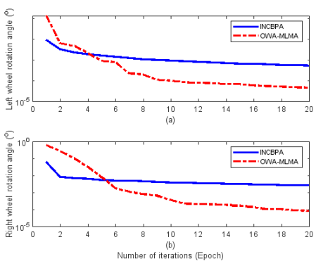
Figure 15. Convergence and minimum performance index comparison of the OWA-MLMA based on AGNA and INCBPA training algorithms for 20 iterations for the NXT robot modeling.
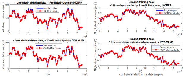
Figure 16. Comparison of one-step ahead output predictions by the trained network (red --*) with the scaled original training data (blue -) for (a) left and (b) right wheel rotation angle angles by OWA-MLMA based on AGNA and INCBPA training algorithms.
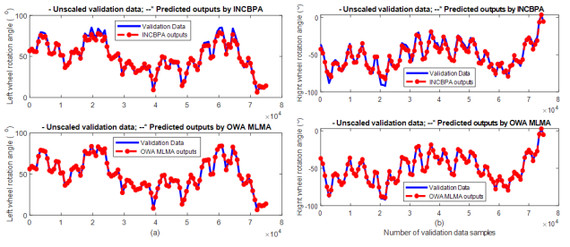
Figure 17. Comparison of one-step ahead output predictions by the trained network (red --*) with the unscaled test data (blue -) for (a) left and (b) right wheel rotation angles by OWA-MLMA based on AGNA and INCBPA training algorithms.
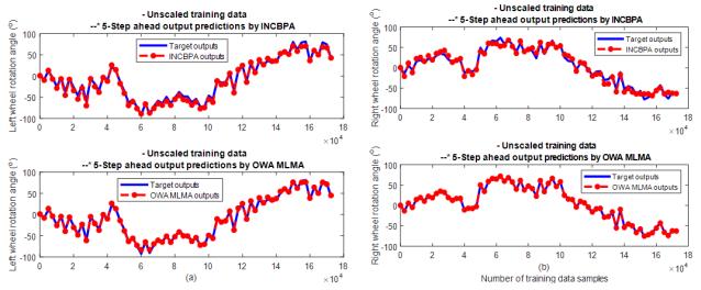
Figure 18. Comparison of 5-step ahead output predictions by the trained network (red --*) with the unscaled original training data (blue -) for (a) left and (b) right wheel rotation angle by OWA-MLMA based on AGNA and INCBPA training algorithms.
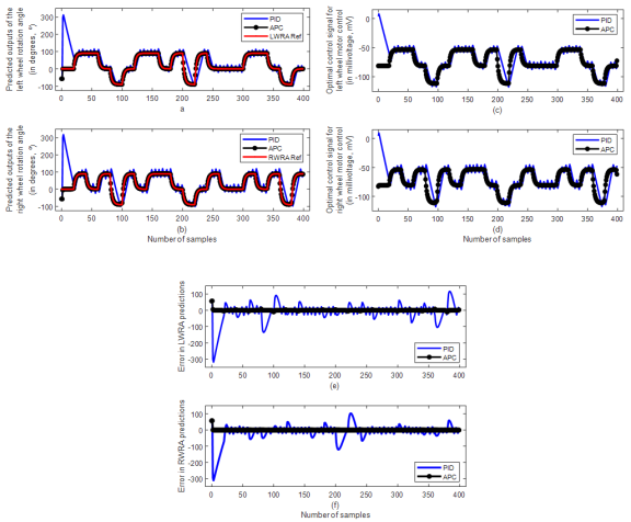
Figure 19. Off-line NXT robot output predictions by PID (blue -) and nonlinear APC (black.-) for (a) LWRA and (b) RWRA with the manipulated signals (c) LWMV and (d) RWMV to track the desired reference signal (red -). Output prediction errors by PID (blue -) and NAPC (black.-) for (e) LWRA) and (f) RWRA.
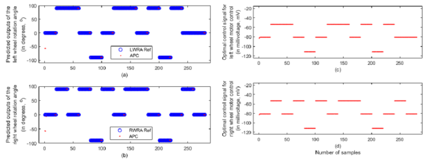
Figure 20. Output predictions for the Online closed-loop implementation of the OWA-MLMA model identification and nonlinear APC based on FNNO-MLMA controller for the NXT robot: reference trajectory (blue o) and NAPC (red.) for (a) LWRA and (b) RWRA with the manipulated signals (c) LWMV and (d) RWMV.
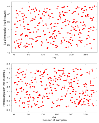
Figure 21. Computation time for the implementation of the OWA-MLMA training algorithm and the nonlinear APC based on FNNO-MLMA control algorithm: (a) series and (b) parallel implementation.
Table 1. Physical parameters, numerical values and units for the self-balancing two-wheeled NXT robot.
Table 2. Iterative Algorithm for Selecting ![]() for Guaranteed Positive Definiteness of the Full Gauss-Newton Hessian Matrix.
for Guaranteed Positive Definiteness of the Full Gauss-Newton Hessian Matrix.
Table 3. Performance comparison of the INCBPA and OWA-MLMA training results.
Table 4. The NXT robot constraints for adaptive control.
Table 5. The NXT robot controller tuning parameters.
Information


 to the error
  in (
in (
 and evaluate
  in (
in ( , compute
  and
and  using (
 , then
  subject to (
 and carry out the recursive computation of the gradient given by (
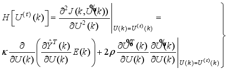
 is given by (
 which is given as:
  in (
in ( given in (
 in (
in ( given in (
 in (
in ( and
and  are the first and second derivatives of (


 ,
,  ,
, ,
,  to
to  in step of
  . Compute (
 to
to 
 or
or  , do
, do to
to  , do
, do to
to  , do
, do
 to
to 
 , Re-compute (
 and
and  , break, end
 , end for
 in (
in ( in (
in ( in (
in ( and compute
  using (
 in (
in (
 , go to Step 9), else go to Step 2).
  in (
in ( in the first term of (