Specific heat, an intrinsic thermal property, represents the amount of heat energy required to raise the temperature of a substance by one degree Celsius. Accurate estimation of specific heat in welded metals is crucial for understanding thermal behavior during and after welding processes, especially in applications where temperature control and energy efficiency are essential. This study focuses on the prediction and optimization of the specific heat of mild steel weldments using Response Surface Methodology (RSM), a statistical technique for modeling and analyzing the effects of multiple variables. A total of 100 welded mild steel specimens, each measuring 60 mm × 40 mm × 10 mm, were prepared through controlled Tungsten Inert Gas (TIG) welding operations. During the experiments, key process parameters - welding current, arc voltage, and shielding gas flow rate - were systematically varied to observe their effect on specific heat. The experimental data collected were analyzed using Design Expert 13 software, enabling statistical modeling, regression analysis, and optimization. A second-order quadratic model was developed to describe the relationship between specific heat and the input parameters. The optimal parameter combination was determined to be 180 A, 19 V, and 13 L/min, resulting in a predicted specific heat value of 445.106 J/kg°C. The developed model provides a useful predictive tool for future thermal analysis of welded structures.
| Published in | Applied Engineering (Volume 9, Issue 1) |
| DOI | 10.11648/j.ae.20250901.13 |
| Page(s) | 37-44 |
| Creative Commons |
This is an Open Access article, distributed under the terms of the Creative Commons Attribution 4.0 International License (http://creativecommons.org/licenses/by/4.0/), which permits unrestricted use, distribution and reproduction in any medium or format, provided the original work is properly cited. |
| Copyright |
Copyright © The Author(s), 2025. Published by Science Publishing Group |
Weldment, Specific Heat, Mild Steel, Temperature, Current, Gas Flow Rate
Independent Variables | Range and Levels of Input Variables | |
|---|---|---|
Lower Range (-1) | Upper Range (+1) | |
Welding Current (Amp) X1 | 150 | 180 |
Welding Voltage (Volt) X2 | 16 | 19 |
Gas flow rate (lit/min) X3 | 13 | 16 |
Std | Run | Current (A) | Voltage (V) | Gas flow rate (lit/min) |
|---|---|---|---|---|
15 | 1 | 165.000 | 17.500 | 14.500 |
16 | 2 | 180.000 | 16.000 | 16.000 |
17 | 3 | 150.000 | 19.000 | 16.000 |
18 | 4 | 165.000 | 17.500 | 14.500 |
19 | 5 | 165.000 | 17.500 | 14.500 |
20 | 6 | 165.000 | 20.023 | 14.500 |
9 | 7 | 180.000 | 19.000 | 16.000 |
10 | 8 | 165.000 | 17.500 | 14.500 |
11 | 9 | 150.000 | 19.000 | 13.000 |
12 | 10 | 165.000 | 17.500 | 14.500 |
13 | 11 | 180.000 | 16.000 | 13.000 |
14 | 12 | 139.773 | 17.500 | 14.500 |
1 | 13 | 180.000 | 19.000 | 13.000 |
2 | 14 | 165.000 | 14.977 | 14.500 |
3 | 15 | 190.227 | 17.500 | 14.500 |
4 | 16 | 165.000 | 17.500 | 11.977 |
5 | 17 | 165.000 | 17.500 | 17.023 |
6 | 18 | 150.000 | 16.000 | 13.000 |
7 | 19 | 150.000 | 16.000 | 16.000 |
8 | 20 | 165.000 | 17.500 | 14.500 |
 (2)
(2) S/N | I, Amp | E, Volt | GFR (Lmin) | Specific heat J/(Kg°C) |
|---|---|---|---|---|
1 | 165.000 | 17.500 | 14.500 | 323.763 |
2 | 180.000 | 16.000 | 16.000 | 357.843 |
3 | 150.000 | 19.000 | 16.000 | 408.963 |
4 | 165.000 | 17.500 | 14.500 | 306.723 |
5 | 165.000 | 17.500 | 14.500 | 323.763 |
6 | 165.000 | 20.023 | 14.500 | 426.004 |
7 | 180.000 | 19.000 | 16.000 | 477.124 |
8 | 165.000 | 17.500 | 14.500 | 306.723 |
9 | 150.000 | 19.000 | 13.000 | 289.682 |
10 | 165.000 | 17.500 | 14.500 | 323.763 |
11 | 180.000 | 16.000 | 13.000 | 340.803 |
12 | 139.773 | 17.500 | 14.500 | 261.816 |
13 | 180.000 | 19.000 | 13.000 | 451.407 |
14 | 165.000 | 14.977 | 14.500 | 312.937 |
15 | 190.227 | 17.500 | 14.500 | 393.636 |
16 | 165.000 | 17.500 | 11.977 | 350.167 |
17 | 165.000 | 17.500 | 17.023 | 424.566 |
18 | 150.000 | 16.000 | 13.000 | 269.086 |
19 | 150.000 | 16.000 | 16.000 | 338.884 |
20 | 165.000 | 17.500 | 14.500 | 318.343 |
Source | Sum of Squares | Df | Mean Square | F-value | p-value | |
|---|---|---|---|---|---|---|
Mean vs Total | 2.454E+06 | 1 | 2.454E+06 | |||
Linear vs Mean | 49959.41 | 3 | 16653.14 | 13.58 | 0.0001 | |
2FI vs Linear | 5521.47 | 3 | 1840.49 | 1.70 | 0.2166 | |
Quadratic vs 2FI | 13221.68 | 3 | 4407.23 | 50.37 | < 0.0001 | Suggested |
Cubic vs Quadratic | 504.76 | 4 | 126.19 | 2.04 | 0.2069 | Aliased |
Residual | 370.24 | 6 | 61.71 | |||
Total | 2.524E+06 | 20 | 1.262E+05 |
Source | Sum of Squares | Df | Mean Square | F-value | p-value | |
|---|---|---|---|---|---|---|
Linear | 19268.09 | 11 | 1751.64 | 25.02 | 0.0012 | |
2FI | 13746.62 | 8 | 1718.33 | 24.54 | 0.0013 | |
Quadratic | 524.93 | 5 | 104.99 | 1.50 | 0.3337 | Suggested |
Cubic | 20.17 | 1 | 20.17 | 0.2882 | 0.6144 | Aliased |
Pure Error | 350.07 | 5 | 70.01 |
Source | Std. Dev. | R² | Adjusted R² | Predicted R² | PRESS | |
|---|---|---|---|---|---|---|
Linear | 35.02 | 0.7180 | 0.6652 | 0.5520 | 31171.42 | |
2FI | 32.93 | 0.7974 | 0.7039 | 0.4845 | 35866.98 | |
Quadratic | 9.35 | 0.9874 | 0.9761 | 0.9308 | 4817.94 | Suggested |
Cubic | 7.86 | 0.9947 | 0.9831 | 0.9288 | 4950.88 | Aliased |
S/N | I, Amp | E, Volt | GFR (Lmin) | Specific heat J/(Kg°C) |
|---|---|---|---|---|
1 | 180.000 | 19.000 | 13.000 | 445.106 |
2 | 179.848 | 19.000 | 13.000 | 444.258 |
3 | 180.000 | 18.987 | 13.000 | 444.350 |
4 | 180.000 | 19.000 | 13.028 | 444.456 |
5 | 180.000 | 19.000 | 13.051 | 443.928 |
6 | 180.000 | 19.000 | 13.062 | 443.671 |
7 | 179.575 | 18.991 | 13.000 | 442.203 |
8 | 179.370 | 19.000 | 13.000 | 441.586 |
9 | 180.000 | 18.959 | 13.000 | 442.802 |
10 | 180.000 | 19.000 | 13.124 | 442.341 |
11 | 180.000 | 19.000 | 16.000 | 475.341 |
12 | 179.870 | 19.000 | 16.000 | 474.928 |
13 | 180.000 | 18.929 | 13.000 | 441.104 |
14 | 180.000 | 19.000 | 15.983 | 474.583 |
15 | 180.000 | 18.983 | 16.000 | 474.233 |
16 | 179.645 | 19.000 | 16.000 | 474.221 |
17 | 180.000 | 18.967 | 16.000 | 473.123 |
18 | 179.416 | 19.000 | 16.000 | 473.500 |
ANOVA | Analysis of Variance |
CCD | Central Composite Design |
DoF | Design of Experiment |
GFR | Gas Flow Rate |
RSM | Response Surface Methodology |
TIG | Tungsten Inert Gas |
VIF | Variance Inflation Factor |
GA | Genetic Algorithm |
| [1] | Callister, W. D., & Rethwisch, D. G. (2018). Materials Science and Engineering: An Introduction (10th ed.). Wiley. |
| [2] | Ferreira, I., Castro, J. A. D., & Garcia, A. (2019). Determination of heat capacity of pure metals, compounds and alloys by analytical and numerical methods. Thermochimica Acta Volume 682, December 2019, 178418. |
| [3] | Parkinson D. H (1958), The specific heats of metals at low temperatures, Reports on Progress in Physics, Volume 21, Number 1. |
| [4] | Jones, H. F. (1957). The specific heat of metals and alloys at low temperatures. Proceedings of the Royal Society of London. Series A. Mathematical and Physical Sciences Volume 240, Issue 1222Jun 1957. |
| [5] | Strombeck, A, Santos, J. F. D., Torster, F. and Koçak, M. (1999) Fracture toughness behavior of FSW joints in aluminium alloys. Proceedings of the I st International Symposium on Friction Stir Welding, 14–16 June, Thousand Oaks, CA, USA. |
| [6] | Galvao, R. M., Leal, D. M., Rodriguez, and Loureiro, A. (2010). Dissimilar welding of very thin aluminum and copper plates. In Proceedings of the 8th International Friction Stir Welding Symposium. Timmendorfer Strand. pp. 1-8. |
| [7] | Zhao, Y., Xie, Q., Zhang, J., Liu, X., and Huang, W. (2020) 'Effect of specific heat on the welding distortion of butt-welded joints', Journal of Materials Processing Technology, Vol. 275, pp. 116317. |
| [8] | Godfrey, S; Tonbra, E (2022), optimization and prediction of melting efficiency of mild steel weldment, using response surface methodology, International Journal of Innovations in Engineering Research and Technology, 9(5), 9. |
| [9] | Igbinake, A. O (2025) comparison of response surface methodology (RSM) and artificial neural networks (ANN) in optimization of the thermal diffusivity of mild steel TIG welding, American Journal of mechanical and material engineering, 2025, vol. 9, No. 2 pp 43-49. |
| [10] | Weman, K; (2011), Welding Processes Handbook, 2nd Edition - November 8, 2011. |
| [11] | Lincoln, E (2014). The Procedure Handbook of Arc Welding 14th ed., page 1.1-1. |
| [12] | Box, G; Behnken, D, (1960) Some new three level designs for the study of quantitative variables, Technometrics, Volume 2, pages 455–475, 1960. |
| [13] | Nuran, B. (2007) The Response Surface Methodology. Master of Science in Applied Mathematics and Computer Science, PhD Dissertation, Faculty of the Indiana University, South Bend. |
| [14] | Sunil C, (2015) ANN and RSM approach for modeling and optimization of designing parameters for a V down perforated baffle roughened rectangular channel Alexandria Engineering Journal Volume 54, Issue 3. |
APA Style
Igbinake, A. O. (2025). Estimation and Optimization of Specific Heat of TIG Weld of Mild Steel (s275) Using Response Surface Methodology. Applied Engineering, 9(1), 37-44. https://doi.org/10.11648/j.ae.20250901.13
ACS Style
Igbinake, A. O. Estimation and Optimization of Specific Heat of TIG Weld of Mild Steel (s275) Using Response Surface Methodology. Appl. Eng. 2025, 9(1), 37-44. doi: 10.11648/j.ae.20250901.13
@article{10.11648/j.ae.20250901.13,
  author = {Augustine Oghenekevwe Igbinake},
  title = {Estimation and Optimization of Specific Heat of TIG Weld of Mild Steel (s275) Using Response Surface Methodology
},
  journal = {Applied Engineering},
  volume = {9},
  number = {1},
  pages = {37-44},
  doi = {10.11648/j.ae.20250901.13},
  url = {https://doi.org/10.11648/j.ae.20250901.13},
  eprint = {https://article.sciencepublishinggroup.com/pdf/10.11648.j.ae.20250901.13},
  abstract = {Specific heat, an intrinsic thermal property, represents the amount of heat energy required to raise the temperature of a substance by one degree Celsius. Accurate estimation of specific heat in welded metals is crucial for understanding thermal behavior during and after welding processes, especially in applications where temperature control and energy efficiency are essential. This study focuses on the prediction and optimization of the specific heat of mild steel weldments using Response Surface Methodology (RSM), a statistical technique for modeling and analyzing the effects of multiple variables. A total of 100 welded mild steel specimens, each measuring 60 mm × 40 mm × 10 mm, were prepared through controlled Tungsten Inert Gas (TIG) welding operations. During the experiments, key process parameters - welding current, arc voltage, and shielding gas flow rate - were systematically varied to observe their effect on specific heat. The experimental data collected were analyzed using Design Expert 13 software, enabling statistical modeling, regression analysis, and optimization. A second-order quadratic model was developed to describe the relationship between specific heat and the input parameters. The optimal parameter combination was determined to be 180 A, 19 V, and 13 L/min, resulting in a predicted specific heat value of 445.106 J/kg°C. The developed model provides a useful predictive tool for future thermal analysis of welded structures.
},
 year = {2025}
}
TY  - JOUR
T1  - Estimation and Optimization of Specific Heat of TIG Weld of Mild Steel (s275) Using Response Surface Methodology

AU  - Augustine Oghenekevwe Igbinake
Y1  - 2025/06/04
PY  - 2025
N1  - https://doi.org/10.11648/j.ae.20250901.13
DO  - 10.11648/j.ae.20250901.13
T2  - Applied Engineering
JF  - Applied Engineering
JO  - Applied Engineering
SP  - 37
EP  - 44
PB  - Science Publishing Group
SN  - 2994-7456
UR  - https://doi.org/10.11648/j.ae.20250901.13
AB  - Specific heat, an intrinsic thermal property, represents the amount of heat energy required to raise the temperature of a substance by one degree Celsius. Accurate estimation of specific heat in welded metals is crucial for understanding thermal behavior during and after welding processes, especially in applications where temperature control and energy efficiency are essential. This study focuses on the prediction and optimization of the specific heat of mild steel weldments using Response Surface Methodology (RSM), a statistical technique for modeling and analyzing the effects of multiple variables. A total of 100 welded mild steel specimens, each measuring 60 mm × 40 mm × 10 mm, were prepared through controlled Tungsten Inert Gas (TIG) welding operations. During the experiments, key process parameters - welding current, arc voltage, and shielding gas flow rate - were systematically varied to observe their effect on specific heat. The experimental data collected were analyzed using Design Expert 13 software, enabling statistical modeling, regression analysis, and optimization. A second-order quadratic model was developed to describe the relationship between specific heat and the input parameters. The optimal parameter combination was determined to be 180 A, 19 V, and 13 L/min, resulting in a predicted specific heat value of 445.106 J/kg°C. The developed model provides a useful predictive tool for future thermal analysis of welded structures.

VL  - 9
IS  - 1
ER  -
Department of Production Engineering, University of Benin, Benin City, Nigeria

Figure 1. Set of equipment for coupon preparation.

Figure 2. Tungsten Inert Gas Welding Equipment.
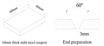
Figure 3. Weld specimen design.
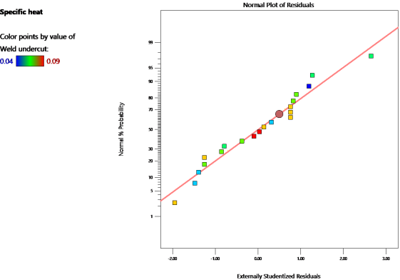
Figure 4. Probability plot of residuals for specific heat.
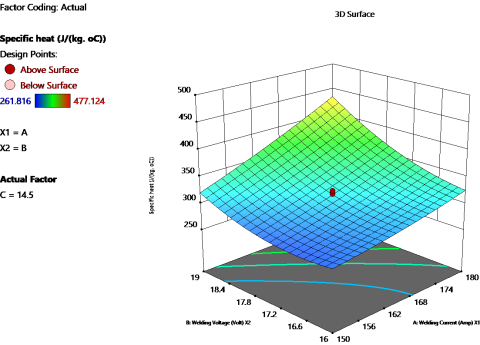
Figure 5. Effect of current and voltage on specific heat.
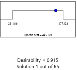
Figure 6. The Ramp plot for Optimization target of specific heat.
Information

