2. Main Contents
2.1. Greedy Facility Location Algorithms Analyzed Using Dual Fitting with Factor-revealing LP
We analyze the first algorithm of Jain, Mahdian
| [4] | Jain, K., Mahdian, M., Markakis, E., Saberi, A. & Vazirani, V. V. (2003). Greedy facility location algorithms analyzed using dual fitting with factor-revealing Lp. J. ACM. |
[4]
and Mahdian, Spielman
| [37] | Mahdian, M., and Spielman, D. A. (2004). Facility location and the analysis of algorithms through factor-revealing programs. Ph. D. Dissertation. Massachusetts Institute of Technology, USA. Order Number: AAI0806252. |
[37]
which has an approximation factor of 1.861, to attempt to solve a real-world case of sitting ULAB collection facilities Mvere
| [1] | E. S. Mvere. (2025) The Near Optimal Siting of Hazardous Waste (Used Lead Acid Battery (ULAB)) Collection Facilities in The Republic of Mauritius Using the Esmvere Cplex k-median solver algorithm. In K. Madhu (Eds,), Advances in Numerical Analysis and Applications. Vol 1, pp, 16-46, ISBN: 978-81-958975-6-8. |
| [2] | E. S. Mvere.(2025) The Near Optimal Siting of Hazardous Waste (Used Lead Acid Battery (ULAB)) Collection Facilities in The Republic of Mauritius Using the ESMVERE Cplex UFL problem solver algorithm. In K. Madhu (Eds,), Advances in Numerical Analysis and Applications. Vol 1, pp, 47-80, ISBN: 978-81-958975-6-8. |
[1, 2]
.
Jain, Vazirani
| [7] | Jain, K. & Vazirani, V. (1999). Primal-dual approximation algorithms for metric facility location and k-median problems. in ‘Proceedings of the 40th Annual Symposium on Foundations of Computer Science’. FOCS ’99. p. 2. |
[7]
proposed a 3 and 6 approximation algorithm for the metric UFL problem and the metric k-median problem, respectively. Their algorithm is an extension of the primary-dual scheme to deal with a primary-dual pair of LPs that are not a covering-packing pair for the UFL metric problem and the k-median metric problem.
To this day, the algorithm they suggest forms the key core basis for all of the primal dual methods. The basic idea behind the algorithm is that each city j continues to boost its dual variable, αj, until it is linked to an open facility, other primary and dual variables simply respond to this transition, trying to preserve feasibility or satisfy complementary conditions of slackness
| [7] | Jain, K. & Vazirani, V. (1999). Primal-dual approximation algorithms for metric facility location and k-median problems. in ‘Proceedings of the 40th Annual Symposium on Foundations of Computer Science’. FOCS ’99. p. 2. |
[7]
.
Jain and Mahdian
| [4] | Jain, K., Mahdian, M., Markakis, E., Saberi, A. & Vazirani, V. V. (2003). Greedy facility location algorithms analyzed using dual fitting with factor-revealing Lp. J. ACM. |
[4]
formalize the methodology used as the dual fitting technique, to examine the set cover problem, Mahdian, Spielman
| [37] | Mahdian, M., and Spielman, D. A. (2004). Facility location and the analysis of algorithms through factor-revealing programs. Ph. D. Dissertation. Massachusetts Institute of Technology, USA. Order Number: AAI0806252. |
[37]
, also introduce the concept of using the approximation factor-revealing LP. Using this duo, Jain and Mahdian
| [4] | Jain, K., Mahdian, M., Markakis, E., Saberi, A. & Vazirani, V. V. (2003). Greedy facility location algorithms analyzed using dual fitting with factor-revealing Lp. J. ACM. |
[4]
analyze two greedy algorithms for the metric UFL problem with 1.861 and 1.61 approximation factors for both problems, respectively, and
and
runtimes, respectively. When explaining the dual fitting method they imply that the basic algorithm is combinatorial, and is a simple greedy algorithm in the case of the set covering problem, assuming it to be a problem of minimization.
Jain and Mahdian
| [4] | Jain, K., Mahdian, M., Markakis, E., Saberi, A. & Vazirani, V. V. (2003). Greedy facility location algorithms analyzed using dual fitting with factor-revealing Lp. J. ACM. |
[4]
describe the combinatorial algorithm as a primal-dual-type algorithm that allows primal and dual updates iteratively, using the problem’s linear programming relaxation and its dual-type algorithm. Although it is not a primal dual algorithm, since the computed dual solution is infeasible, they show that the primal integral solution found by the algorithm is fully paid for by the dual computed solution, meaning that the primal solution’s objective function value is bounded by that of the dual solution
| [4] | Jain, K., Mahdian, M., Markakis, E., Saberi, A. & Vazirani, V. V. (2003). Greedy facility location algorithms analyzed using dual fitting with factor-revealing Lp. J. ACM. |
[4]
. The algorithm’s main step is to divide the dual by a suitable factor,
, and to prove that the shrunk dual is feasible, i.e.
into the instance provided.
On OPT, the shrunk dual is then a lower limit, and
is the approximation guarantee of the algorithm. The aim is therefore to find the necessary minimum
, which is to find the worst possible instance of the problem, one in which the dual solution needs to be shrunk as much as possible in order to make it feasible
| [4] | Jain, K., Mahdian, M., Markakis, E., Saberi, A. & Vazirani, V. V. (2003). Greedy facility location algorithms analyzed using dual fitting with factor-revealing Lp. J. ACM. |
[4]
. Jain and Mahdian
| [4] | Jain, K., Mahdian, M., Markakis, E., Saberi, A. & Vazirani, V. V. (2003). Greedy facility location algorithms analyzed using dual fitting with factor-revealing Lp. J. ACM. |
[4]
describe an approximation factor-revealing LP that encodes the problem of finding the worst possible instance as a linear program.
This provides an LP family, one for each value of the number of cities
. Jain and Mahdian
| [4] | Jain, K., Mahdian, M., Markakis, E., Saberi, A. & Vazirani, V. V. (2003). Greedy facility location algorithms analyzed using dual fitting with factor-revealing Lp. J. ACM. |
[4]
further explain that the best value for
is then the supremum of the optimal solutions to these LP’s. They were unable however, to explicitly measure the supremum, they get a solution which is feasible, to the dual of each of the LP’s. They conjecture that it is possible to determine an upper bound on the duals’ objective function value this is also an upper bound on the optimal
. In the first algorithm, this upper bound is 1.861 and in the second algorithm, 1.61. Jain and Mahdian
| [4] | Jain, K., Mahdian, M., Markakis, E., Saberi, A. & Vazirani, V. V. (2003). Greedy facility location algorithms analyzed using dual fitting with factor-revealing Lp. J. ACM. |
[4]
numerically solves the factor-revealing LP with a large value of
to get a closely matched tight example.
The first algorithm of Jain and Mahdian
| [4] | Jain, K., Mahdian, M., Markakis, E., Saberi, A. & Vazirani, V. V. (2003). Greedy facility location algorithms analyzed using dual fitting with factor-revealing Lp. J. ACM. |
[4]
, is similar to the greedy set cover algorithm, which iteratively selects the most cost-effective choice at each stage. Cost effectiveness is defined as a measure of the ratio of the costs incurred to the number of new cities served. To evaluate this algorithm, they used LP-duality and gave an alternate definition that can be seen as a Jain, Vazirani
| [7] | Jain, K. & Vazirani, V. (1999). Primal-dual approximation algorithms for metric facility location and k-median problems. in ‘Proceedings of the 40th Annual Symposium on Foundations of Computer Science’. FOCS ’99. p. 2. |
[7]
algorithm update.
Algorithm 1 enhances facility location efficiency by balancing opening and connection costs through a structured cost comparison and iterative refinement process. This approach leads to optimized facility placement and city assignment, reducing total operational costs.
The most basic explanation of Jain and Mahdian
| [4] | Jain, K., Mahdian, M., Markakis, E., Saberi, A. & Vazirani, V. V. (2003). Greedy facility location algorithms analyzed using dual fitting with factor-revealing Lp. J. ACM. |
[4]
s first algorithm is, when a city is connected to an open facility, it withdraws everything it has contributed to the opening costs of other facilities, meaning that the dual pays for the primal solution in full.
Jain and Mahdian
| [4] | Jain, K., Mahdian, M., Markakis, E., Saberi, A. & Vazirani, V. V. (2003). Greedy facility location algorithms analyzed using dual fitting with factor-revealing Lp. J. ACM. |
[4]
summarise their first algorithm as:
Let be an unconnected cities set.
All cities are unconnected at the beginning, i.e. := , and all facilities are unopened.
Of all the stars, find the most cost-effective one (, ), open if it’s not already open, and connect all the cities in to
A star consisting of one facility and several cities is defined by Jain and Mahdian
| [4] | Jain, K., Mahdian, M., Markakis, E., Saberi, A. & Vazirani, V. V. (2003). Greedy facility location algorithms analyzed using dual fitting with factor-revealing Lp. J. ACM. |
[4]
. The cost of a star is the sum of the facility’s opening cost and the connection costs between the facility and all the cities in the star in their algorithm. This is formally clarified as the price of a star (
,
), where
is a facility, and
is a subset of cities,
+
. A facility can be selected again after opening in their algorithm, but the opening cost is counted only once and
is set to 0 after the first algorithm selects the facility. When connected to an open facility, each city
is deleted from
and is not taken into account again.
An order is carefully observed with the two algorithms for each facility
, they sort the cities in increasing order of their connection cost to
. Jain and Mahdian
| [4] | Jain, K., Mahdian, M., Markakis, E., Saberi, A. & Vazirani, V. V. (2003). Greedy facility location algorithms analyzed using dual fitting with factor-revealing Lp. J. ACM. |
[4]
determine that a facility and a set containing the first
cities in this order for some
will consist of the most cost-effective star. They describe
as the city
’s contribution or its share of the overall total expenses. They explain how raising the dual variables in each iteration of the greedy algorithm will help find the most cost-effective star.
They restate Algorithm 1 based on the observation that, the most cost-effective star will be the first star (, ) for which =. Dual variables of all unconnected cities are simultaneously increased.
Jain and Mahdian
| [4] | Jain, K., Mahdian, M., Markakis, E., Saberi, A. & Vazirani, V. V. (2003). Greedy facility location algorithms analyzed using dual fitting with factor-revealing Lp. J. ACM. |
[4]
Algorithm 1 restatement:
They add a notion of time, such that each occurrence is related to the time it occurred. The algorithm begins at the moment 0. Each city is initially set to be unconnected (:= ), all facilities are unopened, and is set to 0 for each .
While increases the time and, simultaneously, increases the parameter at the same rate for each city, until one of the incidents below takes place (if two events occur at the same time, they are processed in an arbitrary order).
For some of an unconnected city, and for some of an open facility, =. Connect city to facility and delete from in this case.
We’ve got = for some unopened facility. This ensures that the cities’ total contribution is adequate to open the facility. Open this facility in this case, and with for each of the unconnected cities, connect with , and delete it from .
Jain and Mahdian
| [4] | Jain, K., Mahdian, M., Markakis, E., Saberi, A. & Vazirani, V. V. (2003). Greedy facility location algorithms analyzed using dual fitting with factor-revealing Lp. J. ACM. |
[4]
give an analysis of algorithm 1 in which they explain that every city’s contribution goes into opening one facility at MOST and connecting the city to an open facility. They determine that the total cost of the solution generated by their algorithm is equal to the amount of the
contributions. Jain and Mahdian
| [4] | Jain, K., Mahdian, M., Markakis, E., Saberi, A. & Vazirani, V. V. (2003). Greedy facility location algorithms analyzed using dual fitting with factor-revealing Lp. J. ACM. |
[4]
explain that
is not a feasible dual solution since they remove a subset of cities in each iteration of the restatement of algorithm 1 and withdraw their input from all facilities.
At the end of a facility, therefore,
,
, can be greater than
, thereby violating the corresponding dual constraints. They reiterate that the quest is to find a suitable
for which
is feasible,
will be the lower limit to the optimum, so at most
will be the approximation factor for the algorithm
| [4] | Jain, K., Mahdian, M., Markakis, E., Saberi, A. & Vazirani, V. V. (2003). Greedy facility location algorithms analyzed using dual fitting with factor-revealing Lp. J. ACM. |
[4]
. They include a description that describes that if
is a feasible dual, it is trivial if and only if each facility is
-overtight at most
| [4] | Jain, K., Mahdian, M., Markakis, E., Saberi, A. & Vazirani, V. V. (2003). Greedy facility location algorithms analyzed using dual fitting with factor-revealing Lp. J. ACM. |
[4]
.
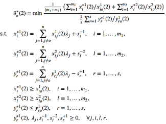
(1)
They conjecture that the goal is to find such a
, and thus the need is to only consider the cities
for which
. Jain and Mahdian
| [4] | Jain, K., Mahdian, M., Markakis, E., Saberi, A. & Vazirani, V. V. (2003). Greedy facility location algorithms analyzed using dual fitting with factor-revealing Lp. J. ACM. |
[4]
give a lemma which captures the metric property:
,
,
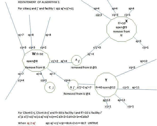
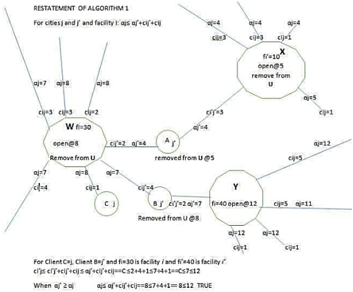
. This lemma is illustrated in the worked example diagrams City A Algorithm 1 and City B Algorithm 1. They state that when
, the inequality obviously holds, as on the diagram City B Algorithm 1.
However as on the diagram City A Algorithm 1 assuming . If city is connected to facility as on the diagram City A Algorithm 1, city A is connected to facility X, fi=10, this facility which is fi=10 on the diagram is open at time which is at 5 on the diagram. The contribution which is 8 on the diagram cannot be greater than which is the distance from client C to facility X, fi=10 on diagram, because in that case city or city C could be connected to facility X, or facility fi= 10 at some time = 5 =8.
Figure 1. City A Algorithm 1.
Figure 2. City B Algorithm 1.
The inequality calculations on Figure 1 serve as a validation step within the algorithm to determine whether a particular city to facility assignment is feasible or optimal based on cost constraints. The inequality compares the sum of connection costs and parameters for two facilities i and i’ with respect to a city j. it checks if the combined cost of assigning city j to facility i’ plus the facility opening cost fi’ is less than or equal to the cost of assigning the same city to facility i plus fi. This helps decide if swtching the city’s assignment to a different facility reduces the overall cost.
The result “UNTRUE” indicates that the assignment is not cost-effective to change under the given parameters. This step is crucial for the algorithm to iteratively refine facility openings and city assignments to minimize total costs in the location optimization problem.
Algoritm 1 improves facility location efficiency by systematically evaluating and optimizing the assignment of cities to facilities based on combined costs, including fixed facility opening costs and connection costs. It calculates the total cost for assigning cities j and j’ to a facility i using the fomular where represents contributions of each city towards opening a facility and represents the connection costs. By comparing these costs across different facilities and cities, the algorithm identifies the most cost-effective assignments, ensuring that facilities with lower total costs are prioritised and opened, while less efficient ones are removed from from the consideration set
The algorithm iteratively opens facilities with the lowest combined costs and removes those that do not improve the overall cost structure, as shown by the removal of facilities W, X and Y from the set U. This selective opening and closing process reduces unnecessary facility openings, minimizing fixed costs while maintaining service quality. The cost comparisons, such as ensure that city assignments are only changed when it leads to a net cost reduction, thus improving allocation efficiency.
Table 1 contains the set of all the cities on the map instance. The map has 16 cities on the first column to the left, On the second column each city is labeled after the facility it is connected to, its nearest facility, either facility W, facility Y or facility X. The city length is the distance between the city and its nearest facility. After a facility opens the city connects to the facility, this is the time it is removed from U, the set of connected facilities.
Table 1.
Restatement of algorithm 1.| [4] | Jain, K., Mahdian, M., Markakis, E., Saberi, A. & Vazirani, V. V. (2003). Greedy facility location algorithms analyzed using dual fitting with factor-revealing Lp. J. ACM. |
U set of cities from Figure 1 | city Label | city length | The time its removed from U |
1 | W1 | 1 | 8 |
2 | W2 | 2 city A | 5 |
3 | W3 | 2 | 8 |
4 | W4 | 3 | 8 |
5 | W5 | 3 | 8 |
6 | W6 | 4 | 8 |
7 | W7 city B | 4 | 8 |
8 | Y1 | 1 | 12 |
9 | Y2 | 1 | 12 |
10 | Y3 | 2 city B | 8 |
11 | Y4 | 5 | 12 |
12 | Y5 | 5 | 11 |
12 | X1 | 1 | 5 |
13 | X2 | 1 | 5 |
14 | X3 | 3 | 5 |
15 | X4 | 3 | 5 |
16 | X5 city A | 3 | 5 |
Table 2. Facility W fi=30.
| t= | W1 | W2 | W3 | W4 | W5 | W6 | W7 | fi contributions |
| | 1 | 2 | 2 | 3 | 3 | 4 | 4 | =19 |
| time | | | | | | | | |
| 0 | 0 | 0 | 0 | 0 | 0 | 0 | 0 | |
0 | 1 | | 1 | 1 | 1 | 1 | 1 | 1 | 0 |
1 | 2 | 1 | | | 1 | 1 | 1 | 1 | 1 |
4 | 3 | 1 | 1 | 1 | | | 1 | 1 | 3 |
9 | 4 | 1 | 1 | 1 | 1 | 1 | | | 5 |
15 | 5 | 1 | 0removed | 1 | 1 | 1 | 1 | 1 | 6 |
21 | 6 | 1 | 0 | 1 | 1 | 1 | 1 | 1 | 6 |
27 | 7 | 1 | 0 | 1 | 1 | 1 | 1 | 1 | 6 |
open 30 | @8 | 1 | 0 | 1 | 1 | - | - | - | 3 |
s | s | 8 | 4 | 8 | 8 | 7 | 7 | 7 | |
Table 2 shows the contribution of each city in terms of
s towards the opening of the Facility W. The
increases as time in seconds, while each connected city contributes towards the opening cost off the facility W. Each city contributes towards covering its distance its distance (cm) first, bold font numbers, when it reaches the facility in distance (cm), then it starts contributing towards the opening of the facility (30 units). When all the contributions from all the cities connected to the facility are equivalent to the opening cost of the facility, the facility opens and connects every city at time 8.
City W2 is connected to another facility from the start of the time facility X, hence when the other facility X opens it connects to it. At time five its removed from U hence it stops contributing towards facility W opening
Table 3. Facility X fi=10.
| t= | X1 | X2 | X3 | X4 | X5 | fi contributions |
| | 1 | 1 | 3 | 3 | 3 | =11 |
| time | | | | | | |
| 0 | 0 | 0 | 0 | 0 | 0 | |
0 | 1 | | | 1 | 1 | 1 | 0 |
2 | 2 | 1 | 1 | 1 | 1 | 1 | 2 |
4 | 3 | 1 | 1 | | | | 2 |
9 | 4 | 1 | 1 | 1 | 1 | 1 | 5 |
Open 10 | @5 | | - | - | - | - | 1 |
s | s | 5 | 4 | 4 | 4 | 4 | |
Table 3 shows the contribution of each city in terms of
s towards the opening of the facility X. The
increases as time in seconds, while each connected city contributes towards the opening cost of the Facility X. Each city contributes towards covering its distance (cm) first, bold font, when it reaches the facility in distance (cm), then it starts contributing towards the opening of the facility (10 units). When all the contributions from all the cities connected to the facility are equivalent to the opening cost of the facility, the facility opens and connects every city at time 5.
Table 4. Facility Y fi=40.
| t= | Y1 | Y2 | Y3 | Y4 | Y5 | fi contributions |
| | 1 | 1 | 2 | 5 | 5 | =14 |
| time | | | | | | |
| 0 | 0 | 0 | 0 | 0 | 0 | 0 |
0 | 1 | | | 1 | 1 | 1 | 0 |
2 | 2 | 1 | 1 | | 1 | 1 | 2 |
5 | 3 | 1 | 1 | 1 | 1 | 1 | 3 |
8 | 4 | 1 | 1 | 1 | 1 | 1 | 3 |
11 | 5 | 1 | 1 | 1 | | | 3 |
16 | 6 | 1 | 1 | 1 | 1 | 1 | 5 |
21 | 7 | 1 | 1 | 1 | 1 | 1 | 5 |
25 | 8 | 1 | 1 | 0removed | 1 | 1 | 4 |
29 | 9 | 1 | 1 | 0 | 1 | 1 | 4 |
33 | 10 | 1 | 1 | 0 | 1 | 1 | 4 |
37 | 11 | 1 | 1 | 0 | 1 | 1 | 4 |
Open 40 | @12 | 1 | 1 | 0 | 1 | - | 3 |
s | s | 12 | 12 | 7 | 12 | 11 | |
Table 4 shows the contributions of each city in terms of
s towards the opening of the Facility Y. The
increases as time in seconds, while each connected city contributes towards the opening cost of the Facility Y. Each city contributes towards covering its distance (cm) first, bold font, when it reaches the facility in distance (cm), then it starts contributing towards the opening of the facility (40 units). When all the contributions from all the cities connected to the facility are equivalent to the opening cost of the facility, the facility opens and connects every city at time 12.
Jain and Mahdian
| [4] | Jain, K., Mahdian, M., Markakis, E., Saberi, A. & Vazirani, V. V. (2003). Greedy facility location algorithms analyzed using dual fitting with factor-revealing Lp. J. ACM. |
[4]
give another lemma which shows how the sum of the
s of every facility must always be below the opening cost. They state this as, during the algorithm, the total contribution provided to a facility at any time is no more than its cost.
. The tables W, X, Y of the worked example diagram Algorithm 1 city B are an example of this. For example Facility W,
, For Facility X,
and For Facility Y,
.
In this lemma Jain and Mahdian
| [4] | Jain, K., Mahdian, M., Markakis, E., Saberi, A. & Vazirani, V. V. (2003). Greedy facility location algorithms analyzed using dual fitting with factor-revealing Lp. J. ACM. |
[4]
give an example of a
for which the
algorithm stops increasing as soon as the
city has a tight edge to a facility which is fully paid for. This means that when a facility opens the algorithm stops increasing the
s thus there is with many facilities at least one
which does not grow to the size of the
. Facility X is an example of this, with city X1 being the
@5 and cities X2, X3, X4, X5 being the
s which stop growing at 4.
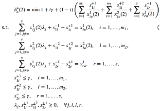
Jain and Mahdian
| [4] | Jain, K., Mahdian, M., Markakis, E., Saberi, A. & Vazirani, V. V. (2003). Greedy facility location algorithms analyzed using dual fitting with factor-revealing Lp. J. ACM. |
[4]
state that the goal is to find the minimum
for which
, hence the maximum of the ratio
is sought.
They go on to state that the maximum value of the objective function of the following program (2) is equal to the Linear Program (7) which they call the factor revealing LP below.
(2)
Subject to the constraints:
(3)
To note this is explained by Facility X where there is a which can be the city larger than all the other cities explained by city XI being the and cities X2, X3, X4, X5 being the ascending s 1,.........., k-1.
(4)
(5)
(6)
The Factor Revealing LP
Subject to the constraints:
(9)
(10)
(11)
(12)
(13)
They state that (Primal):
1) is the optimal solution to the approximation factor-revealing LP.
2) is a lower bound on the value of .
3) is the minimum for which .
4) is the maximum value of the objective function of the ratio .
At optimal, primal and dual solutions are equal thus:
They state that (Dual):
1) A solution to the dual of the approximation actor-revealing LP is needed to prove an upper bound on .
2) An upper bound on the objective function values of the duals of the factor-revealing LP is an upper bound on .
3) It is possible to solve the dual of the factor-revealing LP to prove a close to optimal upper bound on the value of .
The suprenum being the least upper bound, The suprenum of () the optimal solution to the approximatimation factor-revealing LP is the best value of . Therefore =: .
Jain and Mahdian
| [4] | Jain, K., Mahdian, M., Markakis, E., Saberi, A. & Vazirani, V. V. (2003). Greedy facility location algorithms analyzed using dual fitting with factor-revealing Lp. J. ACM. |
[4]
give a lemma for every
1,
1.861.
They multiply the inequalities of the factor-revealing LP to give an inequality of the form:
(14)
(15)
(16)
They suggest that finding the right multipliers for the above inequalities is equivalent to obtaining of the factor-revealing LP. They add three constants , and to prove the bound on for algorithm 1.
(18)
(19)
(21)
(22)
From equation (
18), (
19) and (
20) the inequalities (
16) and (
28) are compared. Inequality (
28) extends inequality (
16) by adding the three constants
,
and
. They denote that the left hand side of inequality (
28) by
and furthermore propose that the sum of the coefficients of
’s in
is at least
. Thus
’s are needed to satisfy the inequality:
(23)
They propose inequality (
23) which guarantees that the average coefficient of
’s in
is at least one. An example of this is the best way to describe the concept: If k is 20, the number of cities being 20.
The total sum of ’s could be 23 therefore
Dividing 23 the total sum of ’s by their number 20 then the average coefficient of ’s is 1.5.
Jain and Mahdian
| [4] | Jain, K., Mahdian, M., Markakis, E., Saberi, A. & Vazirani, V. V. (2003). Greedy facility location algorithms analyzed using dual fitting with factor-revealing Lp. J. ACM. |
[4]
propose that for:
(27)
(28)
They prove that:
in the worst case.
It should be possible, from the look of things by simple analysis, to use an instance created, for the reverse supply chain network design of ULABs in Mauritius, Mvere
| [1] | E. S. Mvere. (2025) The Near Optimal Siting of Hazardous Waste (Used Lead Acid Battery (ULAB)) Collection Facilities in The Republic of Mauritius Using the Esmvere Cplex k-median solver algorithm. In K. Madhu (Eds,), Advances in Numerical Analysis and Applications. Vol 1, pp, 16-46, ISBN: 978-81-958975-6-8. |
| [2] | E. S. Mvere.(2025) The Near Optimal Siting of Hazardous Waste (Used Lead Acid Battery (ULAB)) Collection Facilities in The Republic of Mauritius Using the ESMVERE Cplex UFL problem solver algorithm. In K. Madhu (Eds,), Advances in Numerical Analysis and Applications. Vol 1, pp, 47-80, ISBN: 978-81-958975-6-8. |
[1, 2]
to achieve a solution guaranteed by
. Since γ guarantees that the greedy algorithm Jain and Mahdian
| [4] | Jain, K., Mahdian, M., Markakis, E., Saberi, A. & Vazirani, V. V. (2003). Greedy facility location algorithms analyzed using dual fitting with factor-revealing Lp. J. ACM. |
[4]
solves the UFL problem, (1.861) close to an optimal solution. However, this is not the purpose of this algorithm, and achieving its use in the real world would be extremly difficult and complex. An attempt at this would mean:
1) The instance created for siting ULABs in Mauritius Mvere
| [1] | E. S. Mvere. (2025) The Near Optimal Siting of Hazardous Waste (Used Lead Acid Battery (ULAB)) Collection Facilities in The Republic of Mauritius Using the Esmvere Cplex k-median solver algorithm. In K. Madhu (Eds,), Advances in Numerical Analysis and Applications. Vol 1, pp, 16-46, ISBN: 978-81-958975-6-8. |
| [2] | E. S. Mvere.(2025) The Near Optimal Siting of Hazardous Waste (Used Lead Acid Battery (ULAB)) Collection Facilities in The Republic of Mauritius Using the ESMVERE Cplex UFL problem solver algorithm. In K. Madhu (Eds,), Advances in Numerical Analysis and Applications. Vol 1, pp, 47-80, ISBN: 978-81-958975-6-8. |
[1, 2]
has to be created.
2) To create this instance there is a need to develop a Distance matrix of 156 facilities and 144 clients
3) This n x m would be 22464 distances that have to be measured for each pair of distances between a client and a facility
4) The instance created for siting ULABs in Mauritius
| [1] | E. S. Mvere. (2025) The Near Optimal Siting of Hazardous Waste (Used Lead Acid Battery (ULAB)) Collection Facilities in The Republic of Mauritius Using the Esmvere Cplex k-median solver algorithm. In K. Madhu (Eds,), Advances in Numerical Analysis and Applications. Vol 1, pp, 16-46, ISBN: 978-81-958975-6-8. |
| [2] | E. S. Mvere.(2025) The Near Optimal Siting of Hazardous Waste (Used Lead Acid Battery (ULAB)) Collection Facilities in The Republic of Mauritius Using the ESMVERE Cplex UFL problem solver algorithm. In K. Madhu (Eds,), Advances in Numerical Analysis and Applications. Vol 1, pp, 47-80, ISBN: 978-81-958975-6-8. |
[1, 2]
are encoded as a family of linear programs.
5) The same instance is recreated into a family of instances with different number of nc or cities and clients.
6) Solve these family of LPs created, to get their optimal solutions.
7) Obtain the suprenum of these LPs and compare it to the already known (γ).
8) In each case, with different number of cities nc, we have a usable optimal solution guranteed by (γ).
9) This is because (γ) is the supremum (or the least upper bound) of the optimal solutions to these worst case LP’s.
This has so far proved to be a misconception, an asumption that since the algorithm is well formulated in theory, it can be easily attempted to solve a real world case. Many theoratical science approximation algorithms such as Jain and Mahdian
| [4] | Jain, K., Mahdian, M., Markakis, E., Saberi, A. & Vazirani, V. V. (2003). Greedy facility location algorithms analyzed using dual fitting with factor-revealing Lp. J. ACM. |
[4]
have the most complex transfer from science research to real world application. Approximation algorithms in general can be adapted to specific needs and constraints, they can be used to find multiple solutions, allowing for greater flexibility in decision-making, especially when dealing with real-world problems where constraints and objectives are often "approximately" formulated
| [20] | Chu, C., Antonio, J., (1999) Approximation Algorithms to Solve Real-Life Multicriteria Cutting Stock Problems Operations Research 47: 4, 495-508. |
[20]
. However, not all approximation algorithms are usable practically in real world problems. Some involve complex data structures, or sophisticated algorithmic techniques, leading to difficult implementation issues or improved running time performance (over exact algorithms) only on impractically large inputs
.
In consultation with the Author of
, who is an emminent expert and scolar in the field of theoratical computer science, they revealed that they had not, at the time of writing, implemented their approximation algorithm of
in real world practice, and they were not very familiar with the application side of the two problems, the UFL and the k-median problem. “If you want to implement algorithms for the two problems, you may try to start with the primal-dual algorithms
| [4] | Jain, K., Mahdian, M., Markakis, E., Saberi, A. & Vazirani, V. V. (2003). Greedy facility location algorithms analyzed using dual fitting with factor-revealing Lp. J. ACM. |
[4]
since they do not require you to solve a linear programming”
.
The primal-dual approach in optimization does not always require solving a linear program directly to find a solution
| [18] | Nguyen, K. T.,(2019) Primal-Dual Approaches in Online Algorithms, Algorithmic Game Theory and Online Learning. Operations Research [math. OC]. Université Paris Sorbonne. fftel-02192531f. |
[18]
. It's a powerful technique that constructs feasible primal and dual solutions iteratively, often leading to algorithms where analysis is derived from the primal-dual interaction
| [18] | Nguyen, K. T.,(2019) Primal-Dual Approaches in Online Algorithms, Algorithmic Game Theory and Online Learning. Operations Research [math. OC]. Université Paris Sorbonne. fftel-02192531f. |
[18]
. It focuses on iteratively improving feasible solutions and using the duality relationship to gain insights into the problem, reducing the duality gap, and eventually finding the optimal solution
| [19] | Ebrahimnejad, A.,(2012) A primal-dual method for solving linear programming problems with fuzzy cost coefficients based on linear ranking functions and its applications," International Journal of Industrial and Systems Engineering, Inderscience Enterprises Ltd, vol. 12(2), pages 119-140. |
[19]
. Primal-dual algorithms, avoid explicitly solving a (LP) problem
| [19] | Ebrahimnejad, A.,(2012) A primal-dual method for solving linear programming problems with fuzzy cost coefficients based on linear ranking functions and its applications," International Journal of Industrial and Systems Engineering, Inderscience Enterprises Ltd, vol. 12(2), pages 119-140. |
[19]
. Instead, they construct approximate solutions to the problem and feasible solutions to the dual of an LP relaxation simultaneously
| [22] | Maria, G. L., Hua, W., Henry, W.,(2009). A Stable Primal-Dual Approach for Linear Programming under Nondegeneracy Assumptions. Computational Optimization and Applications. 44. 213-247. https://doi.org/10.1007/s10589-007-9157-2 |
[22]
. This approach leverages the duality relationship between the primal and dual problems, allowing for a more efficient and insightful solution process
| [22] | Maria, G. L., Hua, W., Henry, W.,(2009). A Stable Primal-Dual Approach for Linear Programming under Nondegeneracy Assumptions. Computational Optimization and Applications. 44. 213-247. https://doi.org/10.1007/s10589-007-9157-2 |
[22]
.
2.2. The Near Optimal Siting of Hazardous Waste (Used Lead Acid Battery (ULAB)) Collection Facilities in the Republic of Mauritius Using the | [2] | E. S. Mvere.(2025) The Near Optimal Siting of Hazardous Waste (Used Lead Acid Battery (ULAB)) Collection Facilities in The Republic of Mauritius Using the ESMVERE Cplex UFL problem solver algorithm. In K. Madhu (Eds,), Advances in Numerical Analysis and Applications. Vol 1, pp, 47-80, ISBN: 978-81-958975-6-8. |
[2]
| [1] | E. S. Mvere. (2025) The Near Optimal Siting of Hazardous Waste (Used Lead Acid Battery (ULAB)) Collection Facilities in The Republic of Mauritius Using the Esmvere Cplex k-median solver algorithm. In K. Madhu (Eds,), Advances in Numerical Analysis and Applications. Vol 1, pp, 16-46, ISBN: 978-81-958975-6-8. |
[1]
| [6] | Mvere, E. S (2025). A Systematic Review Of The Esmvere Algorithms, Which Are Contributions In The Field Of Uncapacitated Facility Location Problems And K‐Median Problems International Journal of Science Academic Research, Vol. 06 No. 2, 2025, pp. 9352-9362 |
[6]
Mvere
| [1] | E. S. Mvere. (2025) The Near Optimal Siting of Hazardous Waste (Used Lead Acid Battery (ULAB)) Collection Facilities in The Republic of Mauritius Using the Esmvere Cplex k-median solver algorithm. In K. Madhu (Eds,), Advances in Numerical Analysis and Applications. Vol 1, pp, 16-46, ISBN: 978-81-958975-6-8. |
| [2] | E. S. Mvere.(2025) The Near Optimal Siting of Hazardous Waste (Used Lead Acid Battery (ULAB)) Collection Facilities in The Republic of Mauritius Using the ESMVERE Cplex UFL problem solver algorithm. In K. Madhu (Eds,), Advances in Numerical Analysis and Applications. Vol 1, pp, 47-80, ISBN: 978-81-958975-6-8. |
[1, 2]
explores reverse supply chain network design problems in the automotive industry of the republic of Mauritius, specifically focusing on the challenge of recycling ULABs. The authors examine logistical issues related to the UFL and the k-median location problems
| [6] | Mvere, E. S (2025). A Systematic Review Of The Esmvere Algorithms, Which Are Contributions In The Field Of Uncapacitated Facility Location Problems And K‐Median Problems International Journal of Science Academic Research, Vol. 06 No. 2, 2025, pp. 9352-9362 |
[6]
. Thus Mvere
| [1] | E. S. Mvere. (2025) The Near Optimal Siting of Hazardous Waste (Used Lead Acid Battery (ULAB)) Collection Facilities in The Republic of Mauritius Using the Esmvere Cplex k-median solver algorithm. In K. Madhu (Eds,), Advances in Numerical Analysis and Applications. Vol 1, pp, 16-46, ISBN: 978-81-958975-6-8. |
| [2] | E. S. Mvere.(2025) The Near Optimal Siting of Hazardous Waste (Used Lead Acid Battery (ULAB)) Collection Facilities in The Republic of Mauritius Using the ESMVERE Cplex UFL problem solver algorithm. In K. Madhu (Eds,), Advances in Numerical Analysis and Applications. Vol 1, pp, 47-80, ISBN: 978-81-958975-6-8. |
[1, 2]
deals with the important problem of improving the safety and effectiveness of the collection, processing, and disposal of one of the most hazardous parts of the vehicles, the ULAB
| [6] | Mvere, E. S (2025). A Systematic Review Of The Esmvere Algorithms, Which Are Contributions In The Field Of Uncapacitated Facility Location Problems And K‐Median Problems International Journal of Science Academic Research, Vol. 06 No. 2, 2025, pp. 9352-9362 |
[6]
.
Mvere
| [1] | E. S. Mvere. (2025) The Near Optimal Siting of Hazardous Waste (Used Lead Acid Battery (ULAB)) Collection Facilities in The Republic of Mauritius Using the Esmvere Cplex k-median solver algorithm. In K. Madhu (Eds,), Advances in Numerical Analysis and Applications. Vol 1, pp, 16-46, ISBN: 978-81-958975-6-8. |
| [2] | E. S. Mvere.(2025) The Near Optimal Siting of Hazardous Waste (Used Lead Acid Battery (ULAB)) Collection Facilities in The Republic of Mauritius Using the ESMVERE Cplex UFL problem solver algorithm. In K. Madhu (Eds,), Advances in Numerical Analysis and Applications. Vol 1, pp, 47-80, ISBN: 978-81-958975-6-8. |
[1, 2]
presents a mathematical framework that consists of two facility location problems the UFL, and the k-median problems as alternative approaches to finding the best location sites for the collection facilities of the ULAB batteries Mvere
| [1] | E. S. Mvere. (2025) The Near Optimal Siting of Hazardous Waste (Used Lead Acid Battery (ULAB)) Collection Facilities in The Republic of Mauritius Using the Esmvere Cplex k-median solver algorithm. In K. Madhu (Eds,), Advances in Numerical Analysis and Applications. Vol 1, pp, 16-46, ISBN: 978-81-958975-6-8. |
| [2] | E. S. Mvere.(2025) The Near Optimal Siting of Hazardous Waste (Used Lead Acid Battery (ULAB)) Collection Facilities in The Republic of Mauritius Using the ESMVERE Cplex UFL problem solver algorithm. In K. Madhu (Eds,), Advances in Numerical Analysis and Applications. Vol 1, pp, 47-80, ISBN: 978-81-958975-6-8. |
| [6] | Mvere, E. S (2025). A Systematic Review Of The Esmvere Algorithms, Which Are Contributions In The Field Of Uncapacitated Facility Location Problems And K‐Median Problems International Journal of Science Academic Research, Vol. 06 No. 2, 2025, pp. 9352-9362 |
[1, 2, 6]
present an innovative approach to the siting of hazardous waste collection facilities in Mauritius using the novel ESMVERE CPLEX UFL problem solver algorithm, and the ESMVERE CPLEX k-median problem solver algorithms
| [6] | Mvere, E. S (2025). A Systematic Review Of The Esmvere Algorithms, Which Are Contributions In The Field Of Uncapacitated Facility Location Problems And K‐Median Problems International Journal of Science Academic Research, Vol. 06 No. 2, 2025, pp. 9352-9362 |
[6]
. Both papers address a significant gap in the literature by applying UFL and k-median problem-solving techniques in a real-world setting, using the actual data from the Mauritius statistical office
| [6] | Mvere, E. S (2025). A Systematic Review Of The Esmvere Algorithms, Which Are Contributions In The Field Of Uncapacitated Facility Location Problems And K‐Median Problems International Journal of Science Academic Research, Vol. 06 No. 2, 2025, pp. 9352-9362 |
[6]
. Mvere
| [1] | E. S. Mvere. (2025) The Near Optimal Siting of Hazardous Waste (Used Lead Acid Battery (ULAB)) Collection Facilities in The Republic of Mauritius Using the Esmvere Cplex k-median solver algorithm. In K. Madhu (Eds,), Advances in Numerical Analysis and Applications. Vol 1, pp, 16-46, ISBN: 978-81-958975-6-8. |
| [2] | E. S. Mvere.(2025) The Near Optimal Siting of Hazardous Waste (Used Lead Acid Battery (ULAB)) Collection Facilities in The Republic of Mauritius Using the ESMVERE Cplex UFL problem solver algorithm. In K. Madhu (Eds,), Advances in Numerical Analysis and Applications. Vol 1, pp, 47-80, ISBN: 978-81-958975-6-8. |
[1, 2]
,illustrated a step-by-step instance creation process which familiarizes the reader with how to solve a realistic real-world problem. They clearly demonstrated the algorithm solution to the real-world data from Mauritius using the ArcGIS mapping
| [6] | Mvere, E. S (2025). A Systematic Review Of The Esmvere Algorithms, Which Are Contributions In The Field Of Uncapacitated Facility Location Problems And K‐Median Problems International Journal of Science Academic Research, Vol. 06 No. 2, 2025, pp. 9352-9362 |
[6]
. The solutions are also visible when they are input on google earth
| [6] | Mvere, E. S (2025). A Systematic Review Of The Esmvere Algorithms, Which Are Contributions In The Field Of Uncapacitated Facility Location Problems And K‐Median Problems International Journal of Science Academic Research, Vol. 06 No. 2, 2025, pp. 9352-9362 |
[6]
.
The primary contribution of Mvere
| [1] | E. S. Mvere. (2025) The Near Optimal Siting of Hazardous Waste (Used Lead Acid Battery (ULAB)) Collection Facilities in The Republic of Mauritius Using the Esmvere Cplex k-median solver algorithm. In K. Madhu (Eds,), Advances in Numerical Analysis and Applications. Vol 1, pp, 16-46, ISBN: 978-81-958975-6-8. |
| [2] | E. S. Mvere.(2025) The Near Optimal Siting of Hazardous Waste (Used Lead Acid Battery (ULAB)) Collection Facilities in The Republic of Mauritius Using the ESMVERE Cplex UFL problem solver algorithm. In K. Madhu (Eds,), Advances in Numerical Analysis and Applications. Vol 1, pp, 47-80, ISBN: 978-81-958975-6-8. |
[1, 2]
is the removal of the distance matrix as input in the calculation for the UFL problem and the k-median problem, replacing the distance matrix with the GPS input and Euclidean distance formulae
| [6] | Mvere, E. S (2025). A Systematic Review Of The Esmvere Algorithms, Which Are Contributions In The Field Of Uncapacitated Facility Location Problems And K‐Median Problems International Journal of Science Academic Research, Vol. 06 No. 2, 2025, pp. 9352-9362 |
[6]
. This simplified the data input and reduced computational complexity for the algorithm making it easy, usable, and convenient as a solution
| [6] | Mvere, E. S (2025). A Systematic Review Of The Esmvere Algorithms, Which Are Contributions In The Field Of Uncapacitated Facility Location Problems And K‐Median Problems International Journal of Science Academic Research, Vol. 06 No. 2, 2025, pp. 9352-9362 |
[6]
.
Since their introduction over 60 years ago by Balinsky
| [24] | Balinski, M. (1966). On finding integer solutions to linear programs In: Proceedings of the IBM Scientific Computing Symposium on Combinatorial Problems, pp. 225-248. |
[24]
and Hakimi
| [25] | Hakimi, S. L., (1964). Optimum locations of switching centers and the absolute centers and medians of a graph. Operations Research, 12(3), pp. 450-459. |
[25]
both the UFL and k-median problems have been solved using the distance matrix. Jain, Mahdian
| [4] | Jain, K., Mahdian, M., Markakis, E., Saberi, A. & Vazirani, V. V. (2003). Greedy facility location algorithms analyzed using dual fitting with factor-revealing Lp. J. ACM. |
[4]
, Cacioppi, Watson
| [26] | Cacioppi, P.& Watson, M. (2014). A Deep Dive into Strategic Network Design Programming: OPL CPLEX Edition. Northwestern University Press. |
[26]
, Mistry
, Mahdian, Spielman
| [37] | Mahdian, M., and Spielman, D. A. (2004). Facility location and the analysis of algorithms through factor-revealing programs. Ph. D. Dissertation. Massachusetts Institute of Technology, USA. Order Number: AAI0806252. |
[37]
, are examples of the CPLEX Opl software algorithms that solve the UFL problem using the input of the distance matrix Srinivasan
is a p-median example of how the problems were solved
| [6] | Mvere, E. S (2025). A Systematic Review Of The Esmvere Algorithms, Which Are Contributions In The Field Of Uncapacitated Facility Location Problems And K‐Median Problems International Journal of Science Academic Research, Vol. 06 No. 2, 2025, pp. 9352-9362 |
[6]
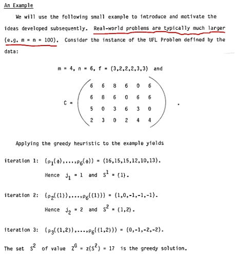
. Cornuejols, Nemhauser
| [29] | Cornuejols, G., Nemhauser, G & Wolsey, L (1984). The Uncapacitated Facility Location Problem. Cornell University |
[29]
is an example of how the UFL problem was solved, as seen on Figure 3.
Thus Mvere
| [1] | E. S. Mvere. (2025) The Near Optimal Siting of Hazardous Waste (Used Lead Acid Battery (ULAB)) Collection Facilities in The Republic of Mauritius Using the Esmvere Cplex k-median solver algorithm. In K. Madhu (Eds,), Advances in Numerical Analysis and Applications. Vol 1, pp, 16-46, ISBN: 978-81-958975-6-8. |
| [2] | E. S. Mvere.(2025) The Near Optimal Siting of Hazardous Waste (Used Lead Acid Battery (ULAB)) Collection Facilities in The Republic of Mauritius Using the ESMVERE Cplex UFL problem solver algorithm. In K. Madhu (Eds,), Advances in Numerical Analysis and Applications. Vol 1, pp, 47-80, ISBN: 978-81-958975-6-8. |
[1, 2]
introduce a solution that does not need the input of a distance matrix but uses GPS based Euclidean distance calculations, while, to the best of our knowledge, all known prior solutions used the input of a distance matrix in the calculation of the UFL problem and the k-median problem
| [6] | Mvere, E. S (2025). A Systematic Review Of The Esmvere Algorithms, Which Are Contributions In The Field Of Uncapacitated Facility Location Problems And K‐Median Problems International Journal of Science Academic Research, Vol. 06 No. 2, 2025, pp. 9352-9362 |
[6]
.
It would be incredibly difficult to use this solution in a real-world scenario, which could explain why there are not so many real-world examples
| [6] | Mvere, E. S (2025). A Systematic Review Of The Esmvere Algorithms, Which Are Contributions In The Field Of Uncapacitated Facility Location Problems And K‐Median Problems International Journal of Science Academic Research, Vol. 06 No. 2, 2025, pp. 9352-9362 |
[6]
. All known prior innovations to the UFL and k-median problem solutions were centered on improvements and innovations around the matrix
| [28] | Srinivasan, G. (2012). Mod-08 Lec-32 Location problems -- p median problem, Fixed charge problem. https://www.youtube.com/watch?v=82OUSjOM2bg pp. 2025–05–26. |
| [29] | Cornuejols, G., Nemhauser, G & Wolsey, L (1984). The Uncapacitated Facility Location Problem. Cornell University |
[28, 29]
. Thus Mvere
| [1] | E. S. Mvere. (2025) The Near Optimal Siting of Hazardous Waste (Used Lead Acid Battery (ULAB)) Collection Facilities in The Republic of Mauritius Using the Esmvere Cplex k-median solver algorithm. In K. Madhu (Eds,), Advances in Numerical Analysis and Applications. Vol 1, pp, 16-46, ISBN: 978-81-958975-6-8. |
| [2] | E. S. Mvere.(2025) The Near Optimal Siting of Hazardous Waste (Used Lead Acid Battery (ULAB)) Collection Facilities in The Republic of Mauritius Using the ESMVERE Cplex UFL problem solver algorithm. In K. Madhu (Eds,), Advances in Numerical Analysis and Applications. Vol 1, pp, 47-80, ISBN: 978-81-958975-6-8. |
[1, 2]
proposes a solution which is a novel breakthrough spanning over 60 years of work in this area
| [24] | Balinski, M. (1966). On finding integer solutions to linear programs In: Proceedings of the IBM Scientific Computing Symposium on Combinatorial Problems, pp. 225-248. |
| [25] | Hakimi, S. L., (1964). Optimum locations of switching centers and the absolute centers and medians of a graph. Operations Research, 12(3), pp. 450-459. |
[24, 25]
. Cacioppi, Watson
| [26] | Cacioppi, P.& Watson, M. (2014). A Deep Dive into Strategic Network Design Programming: OPL CPLEX Edition. Northwestern University Press. |
[26]
, use the distance matrix below (30), in a small nine warehouse example
| [6] | Mvere, E. S (2025). A Systematic Review Of The Esmvere Algorithms, Which Are Contributions In The Field Of Uncapacitated Facility Location Problems And K‐Median Problems International Journal of Science Academic Research, Vol. 06 No. 2, 2025, pp. 9352-9362 |
[6]
. Even in their short example, to ensure that the distance of each point to the other remaining eight points is combinatorically considered, is a big combinatorial task
| [1] | E. S. Mvere. (2025) The Near Optimal Siting of Hazardous Waste (Used Lead Acid Battery (ULAB)) Collection Facilities in The Republic of Mauritius Using the Esmvere Cplex k-median solver algorithm. In K. Madhu (Eds,), Advances in Numerical Analysis and Applications. Vol 1, pp, 16-46, ISBN: 978-81-958975-6-8. |
| [2] | E. S. Mvere.(2025) The Near Optimal Siting of Hazardous Waste (Used Lead Acid Battery (ULAB)) Collection Facilities in The Republic of Mauritius Using the ESMVERE Cplex UFL problem solver algorithm. In K. Madhu (Eds,), Advances in Numerical Analysis and Applications. Vol 1, pp, 47-80, ISBN: 978-81-958975-6-8. |
| [6] | Mvere, E. S (2025). A Systematic Review Of The Esmvere Algorithms, Which Are Contributions In The Field Of Uncapacitated Facility Location Problems And K‐Median Problems International Journal of Science Academic Research, Vol. 06 No. 2, 2025, pp. 9352-9362 |
| [26] | Cacioppi, P.& Watson, M. (2014). A Deep Dive into Strategic Network Design Programming: OPL CPLEX Edition. Northwestern University Press. |
[1, 2, 6, 26]
. This becomes even more complex when you must gather the data between all possible combinations of distances, for example if there are 156 facility locations and 144 client locations
m x
n = 22464 location distances to measure and place in a distance matrix. This is somewhat easy when it is randomly generated by software, however, in real world practice this is extremely complex. Below is a distance matrix of only 9 x 9 locations
| [1] | E. S. Mvere. (2025) The Near Optimal Siting of Hazardous Waste (Used Lead Acid Battery (ULAB)) Collection Facilities in The Republic of Mauritius Using the Esmvere Cplex k-median solver algorithm. In K. Madhu (Eds,), Advances in Numerical Analysis and Applications. Vol 1, pp, 16-46, ISBN: 978-81-958975-6-8. |
| [2] | E. S. Mvere.(2025) The Near Optimal Siting of Hazardous Waste (Used Lead Acid Battery (ULAB)) Collection Facilities in The Republic of Mauritius Using the ESMVERE Cplex UFL problem solver algorithm. In K. Madhu (Eds,), Advances in Numerical Analysis and Applications. Vol 1, pp, 47-80, ISBN: 978-81-958975-6-8. |
| [6] | Mvere, E. S (2025). A Systematic Review Of The Esmvere Algorithms, Which Are Contributions In The Field Of Uncapacitated Facility Location Problems And K‐Median Problems International Journal of Science Academic Research, Vol. 06 No. 2, 2025, pp. 9352-9362 |
[1, 2, 6]
.
Cacioppi, Watson
| [26] | Cacioppi, P.& Watson, M. (2014). A Deep Dive into Strategic Network Design Programming: OPL CPLEX Edition. Northwestern University Press. |
[26]
Distance Matrix (30)
];
This would be impractical in many cases in the real world where there might be hundreds or thousands of location points, and the distances that make each pair of distances
| [1] | E. S. Mvere. (2025) The Near Optimal Siting of Hazardous Waste (Used Lead Acid Battery (ULAB)) Collection Facilities in The Republic of Mauritius Using the Esmvere Cplex k-median solver algorithm. In K. Madhu (Eds,), Advances in Numerical Analysis and Applications. Vol 1, pp, 16-46, ISBN: 978-81-958975-6-8. |
| [2] | E. S. Mvere.(2025) The Near Optimal Siting of Hazardous Waste (Used Lead Acid Battery (ULAB)) Collection Facilities in The Republic of Mauritius Using the ESMVERE Cplex UFL problem solver algorithm. In K. Madhu (Eds,), Advances in Numerical Analysis and Applications. Vol 1, pp, 47-80, ISBN: 978-81-958975-6-8. |
| [6] | Mvere, E. S (2025). A Systematic Review Of The Esmvere Algorithms, Which Are Contributions In The Field Of Uncapacitated Facility Location Problems And K‐Median Problems International Journal of Science Academic Research, Vol. 06 No. 2, 2025, pp. 9352-9362 |
[1, 2, 6]
. Thus, a new model is developed that does not need the input of the distance matrix but uses the formulae for the Euclidean distance between two points and the input of actual GPS coordinate location points to solve the UFL and the k-median problem in Mvere
| [1] | E. S. Mvere. (2025) The Near Optimal Siting of Hazardous Waste (Used Lead Acid Battery (ULAB)) Collection Facilities in The Republic of Mauritius Using the Esmvere Cplex k-median solver algorithm. In K. Madhu (Eds,), Advances in Numerical Analysis and Applications. Vol 1, pp, 16-46, ISBN: 978-81-958975-6-8. |
| [2] | E. S. Mvere.(2025) The Near Optimal Siting of Hazardous Waste (Used Lead Acid Battery (ULAB)) Collection Facilities in The Republic of Mauritius Using the ESMVERE Cplex UFL problem solver algorithm. In K. Madhu (Eds,), Advances in Numerical Analysis and Applications. Vol 1, pp, 47-80, ISBN: 978-81-958975-6-8. |
| [6] | Mvere, E. S (2025). A Systematic Review Of The Esmvere Algorithms, Which Are Contributions In The Field Of Uncapacitated Facility Location Problems And K‐Median Problems International Journal of Science Academic Research, Vol. 06 No. 2, 2025, pp. 9352-9362 |
[1, 2, 6]
. This solution is user friendly and convenient.
The formula for the Euclidean distance between two points is:
The UFL, k-median CPLEX Opl Euclidean distance formulae developed for this study by Mvere
| [1] | E. S. Mvere. (2025) The Near Optimal Siting of Hazardous Waste (Used Lead Acid Battery (ULAB)) Collection Facilities in The Republic of Mauritius Using the Esmvere Cplex k-median solver algorithm. In K. Madhu (Eds,), Advances in Numerical Analysis and Applications. Vol 1, pp, 16-46, ISBN: 978-81-958975-6-8. |
| [2] | E. S. Mvere.(2025) The Near Optimal Siting of Hazardous Waste (Used Lead Acid Battery (ULAB)) Collection Facilities in The Republic of Mauritius Using the ESMVERE Cplex UFL problem solver algorithm. In K. Madhu (Eds,), Advances in Numerical Analysis and Applications. Vol 1, pp, 47-80, ISBN: 978-81-958975-6-8. |
| [6] | Mvere, E. S (2025). A Systematic Review Of The Esmvere Algorithms, Which Are Contributions In The Field Of Uncapacitated Facility Location Problems And K‐Median Problems International Journal of Science Academic Research, Vol. 06 No. 2, 2025, pp. 9352-9362 |
[1, 2, 6]
:
{
The new method solves the UFL and the k-median problem by making a choice between facility locations and client locations, without considering the distance between all the points as a distance matrix
| [6] | Mvere, E. S (2025). A Systematic Review Of The Esmvere Algorithms, Which Are Contributions In The Field Of Uncapacitated Facility Location Problems And K‐Median Problems International Journal of Science Academic Research, Vol. 06 No. 2, 2025, pp. 9352-9362 |
[6]
. The newly developed method only requires the GPS coordinate location points
| [1] | E. S. Mvere. (2025) The Near Optimal Siting of Hazardous Waste (Used Lead Acid Battery (ULAB)) Collection Facilities in The Republic of Mauritius Using the Esmvere Cplex k-median solver algorithm. In K. Madhu (Eds,), Advances in Numerical Analysis and Applications. Vol 1, pp, 16-46, ISBN: 978-81-958975-6-8. |
| [2] | E. S. Mvere.(2025) The Near Optimal Siting of Hazardous Waste (Used Lead Acid Battery (ULAB)) Collection Facilities in The Republic of Mauritius Using the ESMVERE Cplex UFL problem solver algorithm. In K. Madhu (Eds,), Advances in Numerical Analysis and Applications. Vol 1, pp, 47-80, ISBN: 978-81-958975-6-8. |
| [6] | Mvere, E. S (2025). A Systematic Review Of The Esmvere Algorithms, Which Are Contributions In The Field Of Uncapacitated Facility Location Problems And K‐Median Problems International Journal of Science Academic Research, Vol. 06 No. 2, 2025, pp. 9352-9362 |
[1, 2, 6]
. This means that it opens the best out of
n potential facility locations and assigns only
m clients to these open facilities per calculation
| [1] | E. S. Mvere. (2025) The Near Optimal Siting of Hazardous Waste (Used Lead Acid Battery (ULAB)) Collection Facilities in The Republic of Mauritius Using the Esmvere Cplex k-median solver algorithm. In K. Madhu (Eds,), Advances in Numerical Analysis and Applications. Vol 1, pp, 16-46, ISBN: 978-81-958975-6-8. |
| [2] | E. S. Mvere.(2025) The Near Optimal Siting of Hazardous Waste (Used Lead Acid Battery (ULAB)) Collection Facilities in The Republic of Mauritius Using the ESMVERE Cplex UFL problem solver algorithm. In K. Madhu (Eds,), Advances in Numerical Analysis and Applications. Vol 1, pp, 47-80, ISBN: 978-81-958975-6-8. |
| [6] | Mvere, E. S (2025). A Systematic Review Of The Esmvere Algorithms, Which Are Contributions In The Field Of Uncapacitated Facility Location Problems And K‐Median Problems International Journal of Science Academic Research, Vol. 06 No. 2, 2025, pp. 9352-9362 |
[1, 2, 6]
.
A combination of the CPLEX solutions to the Travelling Salesman Problem (TSP) by Caceres
and a CPLEX solution to the p-median algorithm by Cacioppi, Watson
| [26] | Cacioppi, P.& Watson, M. (2014). A Deep Dive into Strategic Network Design Programming: OPL CPLEX Edition. Northwestern University Press. |
[26]
, was used to develop a new and unique software invention which solves the UFL and k-median problem by Mvere [1 ,2 ,6]. The works of Cacioppi, Watson
| [26] | Cacioppi, P.& Watson, M. (2014). A Deep Dive into Strategic Network Design Programming: OPL CPLEX Edition. Northwestern University Press. |
[26]
and Caceres
were thoroughly analyzed and reviewed.
Combining these two solutions made it possible to develop 3 entirely new CPLEX models which solve the UFL problem, k-UFL problem and k-median problem
| [6] | Mvere, E. S (2025). A Systematic Review Of The Esmvere Algorithms, Which Are Contributions In The Field Of Uncapacitated Facility Location Problems And K‐Median Problems International Journal of Science Academic Research, Vol. 06 No. 2, 2025, pp. 9352-9362 |
[6]
. The sub tour elimination decision variables of the TSP problem were removed
. Arrays of the facility locations and opening costs were added in Mvere
| [1] | E. S. Mvere. (2025) The Near Optimal Siting of Hazardous Waste (Used Lead Acid Battery (ULAB)) Collection Facilities in The Republic of Mauritius Using the Esmvere Cplex k-median solver algorithm. In K. Madhu (Eds,), Advances in Numerical Analysis and Applications. Vol 1, pp, 16-46, ISBN: 978-81-958975-6-8. |
| [2] | E. S. Mvere.(2025) The Near Optimal Siting of Hazardous Waste (Used Lead Acid Battery (ULAB)) Collection Facilities in The Republic of Mauritius Using the ESMVERE Cplex UFL problem solver algorithm. In K. Madhu (Eds,), Advances in Numerical Analysis and Applications. Vol 1, pp, 47-80, ISBN: 978-81-958975-6-8. |
| [6] | Mvere, E. S (2025). A Systematic Review Of The Esmvere Algorithms, Which Are Contributions In The Field Of Uncapacitated Facility Location Problems And K‐Median Problems International Journal of Science Academic Research, Vol. 06 No. 2, 2025, pp. 9352-9362 |
[1, 2, 6]
, these enabled the costs of the edges to be computed from each facility to each client. The changes have developed entirely new software solutions in Mvere
| [6] | Mvere, E. S (2025). A Systematic Review Of The Esmvere Algorithms, Which Are Contributions In The Field Of Uncapacitated Facility Location Problems And K‐Median Problems International Journal of Science Academic Research, Vol. 06 No. 2, 2025, pp. 9352-9362 |
[6]
after careful consideration and study.
Definition of parameters
a) is used to denote a (ulab collection facility).
b) is used to denote a (ulab city) it is a residential area with a population of clients that want to dispose ulabs in Mauritius.
c) is a decision variable which denotes whether (ulab collection facility) is connected to (ulab city) or not. is a binary variable, which becomes 1 if (ulab collection facility) is connected to (ulab city) or 0 if (ulab collection facility) is not connected. Being connected means the (ulab city) can dispose its ulabs at the open (ulab collection facility).
d) is a decision variable which denotes whether (ulab collection facility) is open or not. is a binary variable, which becomes 1 if (ulab collection facility) is open to receive disposed ulabs from (ulab cities), or 0 if (ulab collection facility) is not open to receive ulabs.
e) denotes the cost of the distance from (ulab city) to (ulab collection facility) . The distance determines the cost which has to be minimized. The distance is only a significant cost if the (ulab collection facility) is open and connected to (ulab city) , that is if is 1.
f) is the larger set of (ulab collection facilities). The goal is to open the best set of (ulab collection facilities), which serve all the (ulab cities) at a minimum cost. The best set of (ulab collection facilities) is chosen and opened from the larger set of (ulab collection facilities).
g) is the larger set of (ulab cities). All the (ulab cities) have to be served and Connected to a (ulab collection facility). All the (ulab cities) have to be connected to an open (ulab collection facilities), Unlike and direct opposite of (ulab collection facilities, where there is a choice to select the optimum located, open them, and let the rest remain closed.
h) is the best set of (ulab collection facilities) opened. This is when the best set of (ulab collection facilities) is chosen and opened from the larger set of potential (ulab collection facilities).
i) the costs of opening (ulab collection facilities) . The facility opening cost is one of the variables that determines the final value of the objective function. The objective is to minimize the sum of the (ulab collection facilities) opening costs.
The metric UFL problem is formulated as an integer program to satisfy the constraints:
(32)
Subject to the constraints:
The mathematical formulation of the UFL problem is then converted to the CPLEX Opl language. The model formulation is translated into the Opl language using the IBM ILOG CPLEX Optimization Studio IDE 20.1.0. Exactly as the TSP model by Caceres
described in the literature the CPLEX Optimization Engine requires a model of the form:
1. Size or Range
2. Input Data Sources
3. Decision Variables
4. Decision Expressions
5. Objective Function
6. Constraints
1) Size or Range
The Opl language is used to declare two integer variables is for the (ulab collection facilities) and is for the (ulab cities). The Opl language is used to create two range variables and which contain all the (ulab collection facilities) and (ulab cities) on the plane.
// is the number of (ulab collection facilities)
// is the number of (ulab cities)
//the range of all the facilities from 1 up to n.
//the range of all the cities from 1 up to m.
//this is an array of the opening costs of all (ulab collection facilities)
In the CPLEX data file //the opening costs of all (ulab collection facilities) are given as a matrix:
2) Input Data Sources
The tuple is created for this model, this contains the float variables and . When it is called, this method divides the plane into and coordinates. It gives the location of every (ulab collection facility) and (ulab city). It also gives the starting and ending point of every edge, in terms of its and coordinates.
The tuple is created, this contains the integer variables and . When it is called, this method connects all the points on the plane into edges, and every edge has beginning point (ulab city) and ending point (ulab collection facility) . Thus, the tuple is called to create the edges.
A set of edges named is created, which defines the character of what an edge is, and defines its boundaries, while placing all the edges on the plane into a set. The edge is described as less than the variable and greater than the variable , is found in the and is within the .
A float variable is created, this is an array variable. is an array of all the edges from the variable which contains the set of all the edges. Square braces are used to denote an array and in this case are used to describe the variable as an array which contains the set of all edges .
The tuple is called to create an array which contains the range . This array places and coordinates in every city. The array stores the and coordinates of every city.
The tuple is called to create an array which contains the range . This array places and coordinates on every facility. The array stores the and coordinates of every facility.
The generated data is preprocessed before the problem is computed. To preprocess the data, a code block
is created. In the code block, a
is declared, this function calculates and returns the Euclidean 2-dimensional distance between a facility and a city. It returns this value based on their
and
coordinates. The formula for the Euclidean distance between two points is the same as on formular (
31)
calculated by subtracting the coordinates of the two points and the result squared is added to the subtraction of the two coordinates of the two points. The difference of the subtraction of the two points were the coordinates are subtracting each other and the coordinates are subtracting each other is squared and then it is added. The square root of this difference is the length of the distance. This general common formula is translated into the Opl Language in the function illustrated in the code below.
In the code block , a for loop which randomly generates the and coordinates of every ulabcity are created as well as a for loop which randomly generates the and coordinates of every ulabfacility. Finally in the same code block , a for loop with a variable is constructed. represents every edge in the set of . The loop goes to the array which is an array which stores all the edges from the variable which contains the set of all the edges, it then uses the to calculate the size of every edge in terms of the and coordinates of its starting point the ulabcity and its ending point the ulabfacility .
The code block above, which is written in the Opl Language, contains one function and three for loops. The function returns the Euclidean 2-dimensional distance between two points.
The first for loop in the code block is created by declaring a variable . The variable loops through every (ulab collection facility), in the range . It places and coordinates. The code searches for an coordinate from the array in the data file. it loops through all the (ulab collection facilities) in the array. The code searches for an coordinate from the array looping through every (ulab collection facility) in the array.
The second for loop in the code block is created by declaring a variable . The variable loops through every (ulab city), in the range . It places and coordinates. The code searches for an coordinate from the array in the data file. it loops through all the (ulabcities) in the array. The code searches for an coordinate from the array looping through every (ulab city) in the array.
The third for loop in the code block is created by declaring a variable . The variable loops through every edge in the set of edges. The function then calculates the distance between the and coordinates of the and the and coordinates of the of each edge. Each edge has beginning point and ending point . The function returns this distance for each edge in the array of edges . This just gives the length of every edge on the plane.
3) Decision Variables
There are two main decision variables in the UFL problem , which is declared in CPLEX Opl in the model as a Boolean decision variable
, then there is which is also declared in the model as a Boolean decision variable
The two variables stand for the solution set of facilities and edges. The variable is multiplied to an element of an array . The array that the variable is multiplied to, is an array of the tuple . The elements of the tuple are the contents of the array . Thus, the tuple contains integer variables ’s and ’s. Therefore connects ’s and ’s in an array to create the edges.
4) Decision Expressions
Decision variables and decision expressions are used to create the actual Opl model. Caceres
translate the mathematical formulation of the model decision expression into the Opl language.
(37)
The two decision expressions have been placed above and below, to compare and juxtapose the translation so that other models can also be analyzed and translated into the Opl language model.
5) Objective Function
The objective function is that of the UFL problem in that it is to minimize the total sum of opening costs, and the total distance traveled from (ulabcity) to (ulabfacility) location.
6) Constraints
The constraints are translated from the mathematical formulation of the UFL problem into Opl as a code block . In the constraint code block , the first constraint is placed as a for loop.
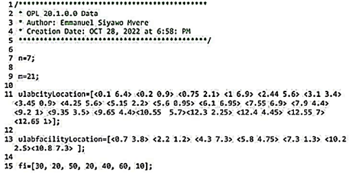
7) The Data
The CPLEX data file contains the data values which are entered manually. The values of the number of (ulabfacilities), the number of ulabcities. It also contains the values of the two arrays, and which host the and coordinates of ulabcity locations and ulab collection facility locations. It also contains the values of the array in which is entered the opening cost values of the ulab collection facilities.
8) The Input File
The location input is within an array of x and y coordinates ulabcitylocation and ulabfacilityLocation: [<x y> <x y>] can be replaced by GPS Coordinates for example: [< -20.172544 57.4883317 > <-20.165595 57.492625>]. The input coordinates are easier and more convenient to input for the calculation of the UFL problem compared with a distance matrix of the same coordinate points. This makes the algorithm solution user friendly, and usable in a real-world case.
Li
shows an example problem where Walmart tasks the k-median problem, Mvere
| [1] | E. S. Mvere. (2025) The Near Optimal Siting of Hazardous Waste (Used Lead Acid Battery (ULAB)) Collection Facilities in The Republic of Mauritius Using the Esmvere Cplex k-median solver algorithm. In K. Madhu (Eds,), Advances in Numerical Analysis and Applications. Vol 1, pp, 16-46, ISBN: 978-81-958975-6-8. |
[1]
, an American retail giant, to select the best locations to site their retail stores. The aim was to site their 50 stores in Washington state so that the average travelling time for people to their nearest Walmart shop is minimized
. This is an example of a real-world case where the average travelling time, distance, is minimized. However, the decision is only concentrated on financial terms, monetized terms
| [1] | E. S. Mvere. (2025) The Near Optimal Siting of Hazardous Waste (Used Lead Acid Battery (ULAB)) Collection Facilities in The Republic of Mauritius Using the Esmvere Cplex k-median solver algorithm. In K. Madhu (Eds,), Advances in Numerical Analysis and Applications. Vol 1, pp, 16-46, ISBN: 978-81-958975-6-8. |
| [2] | E. S. Mvere.(2025) The Near Optimal Siting of Hazardous Waste (Used Lead Acid Battery (ULAB)) Collection Facilities in The Republic of Mauritius Using the ESMVERE Cplex UFL problem solver algorithm. In K. Madhu (Eds,), Advances in Numerical Analysis and Applications. Vol 1, pp, 47-80, ISBN: 978-81-958975-6-8. |
[1, 2]
. There are other criteria such as competition with other retail stores within the vicinity, the presence of other buildings, residential areas, road density, population density and demographics and other factors that are not put into consideration with location models like Mvere
| [1] | E. S. Mvere. (2025) The Near Optimal Siting of Hazardous Waste (Used Lead Acid Battery (ULAB)) Collection Facilities in The Republic of Mauritius Using the Esmvere Cplex k-median solver algorithm. In K. Madhu (Eds,), Advances in Numerical Analysis and Applications. Vol 1, pp, 16-46, ISBN: 978-81-958975-6-8. |
| [2] | E. S. Mvere.(2025) The Near Optimal Siting of Hazardous Waste (Used Lead Acid Battery (ULAB)) Collection Facilities in The Republic of Mauritius Using the ESMVERE Cplex UFL problem solver algorithm. In K. Madhu (Eds,), Advances in Numerical Analysis and Applications. Vol 1, pp, 47-80, ISBN: 978-81-958975-6-8. |
[1, 2]
and Jain, Mahdian
| [4] | Jain, K., Mahdian, M., Markakis, E., Saberi, A. & Vazirani, V. V. (2003). Greedy facility location algorithms analyzed using dual fitting with factor-revealing Lp. J. ACM. |
[4]
which may affect the performance of the Walmart store when it is located on any optimally selected facility location by the UFL or k-median problem.
The DEA and TOPSIS method may be used in Location analysis to make an informed decision in such a case as suggested by Li
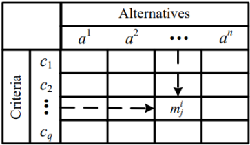
which includes many other criteria. Each of the 50 locations is turned into a DMU and listed as an alternative, its performance as a potential location is evaluated according to the multiple criteria. This involves a lot of data gathering. It also involves a lot of subjective choices and preferences of the decision makers and the community.
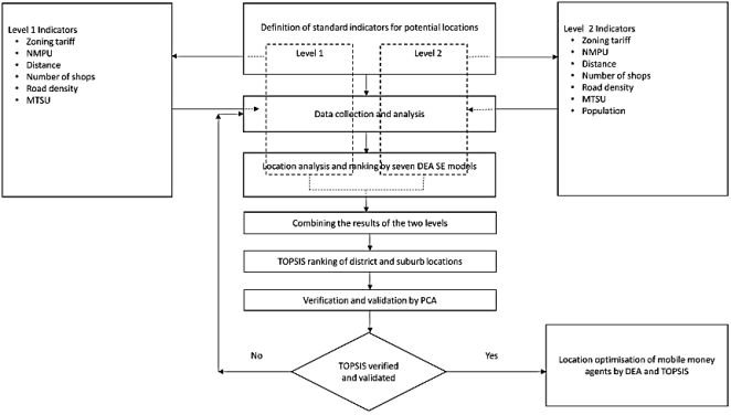
2.3. Hierarchical Groups DEA Super-efficiency and Group TOPSIS Technique: Application on Mobile Money Agents’ Locations
Multi Criteria Decision Analysis (MCDA) is the umbrella term for methods that deal with multiple criteria, while DEA and TOPSIS are specific tools within that framework. They all contribute to the process of making informed decisions when there are multiple factors to consider
| [15] | Charles, V., Aparicio, J., Zhu, J.(2019) The curse of dimensionality of decision-making units: A simple approach to increase the discriminatory power of data envelopment analysis, European Journal of Operational Research, Volume 279, Issue 3, Pages 929-940, ISSN 0377-2217, |
[15]
. While DEA is a non-parametric method used to evaluate the relative efficiency of DMUs, which are entities that convert inputs into outputs
| [33] | Labijak-Kowalska, A., Kadziński, M., & Mrozek, W. (2023). Robust Additive Value-Based Efficiency Analysis with a Hierarchical Structure of Inputs and Outputs. Applied Sciences, 13(11), 6406. https://doi.org/10.3390/app13116406 |
[33]
. TOPSIS ranks alternatives based on their distance to both an ideal solution and a non-ideal solution
| [16] | Ramdania, D. R., Manaf, K., Junaedi, F. R., Fathonih, A., Hadiana, A,(2020) TOPSIS Method on Selection of New Employees’ Acceptance,"6th International Conference on Wireless and Telematics (ICWT), Yogyakarta, pp. 1-4, https://doi.org/10.1109/ICWT50448.2020.9243658 |
[16]
. In location analysis, DEA and TOPSIS were used by Muvingi, Peer
| [3] | Muvingi, J., Peer, A. A. I., Hosseinzadeh Lotfi, F., & Ozsoy, V. S. (2023). Hierarchical groups DEA super-efficiency and group TOPSIS technique: Application on mobile money agents’ locations, Expert Systems with Applications, Volume 234, 0957-4174, https://doi.org/10.1016/j.eswa.2023.121033 |
| [32] | Muvingi, J., Peer, A. A. I., Hosseinzadeh Lotfi, F., & Ozsoy, V. S. (2022). Hierarchical groups DEA cross-efficiency and TOPSIS technique: An application on mobile money agents locations. International Journal of Mathematics in Operational Research, 21(2), 171–199. http://dx.doi.org/10.1504/IJMOR.2020.10037455 |
[3. 32]
, Chen, Li
and Zangeneh, Akram
| [31] | Zangeneh, M., Akram, A., Nielsen, P., Keyhani, A., & Banaeian, N. (2015). A solution approach for agricultural service center location problems using TOPSIS, DEA and SAW techniques. In P. Golinska, & A. Kawa (Eds.), Technology management for sustainable production and logistics (pp. 25–56). Springer, Berlin, Heidelberg, http://dx.doi.org/10.1007/978-3-642-33935-6_2 |
[31]
.
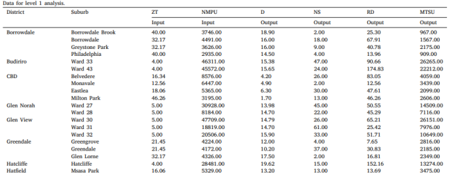
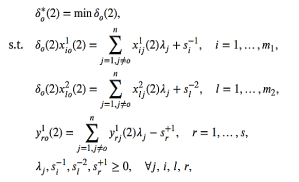
Hierarchical groups DEA super-efficiency refers to a method used in (DEA) to assess the efficiency of DMUs that have a hierarchical structure, where some DMUs are part of larger groups, for example districts and suburbs
| [3] | Muvingi, J., Peer, A. A. I., Hosseinzadeh Lotfi, F., & Ozsoy, V. S. (2023). Hierarchical groups DEA super-efficiency and group TOPSIS technique: Application on mobile money agents’ locations, Expert Systems with Applications, Volume 234, 0957-4174, https://doi.org/10.1016/j.eswa.2023.121033 |
[3]
.
It extends the concept of super-efficiency, which is used to rank and compare DMUs that are already efficient in the traditional DEA analysis
| [3] | Muvingi, J., Peer, A. A. I., Hosseinzadeh Lotfi, F., & Ozsoy, V. S. (2023). Hierarchical groups DEA super-efficiency and group TOPSIS technique: Application on mobile money agents’ locations, Expert Systems with Applications, Volume 234, 0957-4174, https://doi.org/10.1016/j.eswa.2023.121033 |
[3]
. Super-efficiency methods are used to rank and compare efficient units. DEA determines a "best-practice frontier" by identifying the most efficient DMUs and then compares other DMUs against this frontier
| [33] | Labijak-Kowalska, A., Kadziński, M., & Mrozek, W. (2023). Robust Additive Value-Based Efficiency Analysis with a Hierarchical Structure of Inputs and Outputs. Applied Sciences, 13(11), 6406. https://doi.org/10.3390/app13116406 |
| [35] | Bajec, P., Tuljak-Suban, D., & Zalokar, E. (2021). A Distance-Based AHP-DEA Super-Efficiency Approach for Selecting an Electric Bike Sharing System Provider: One Step Closer to Sustainability and a Win–Win Effect for All Target Groups. Sustainability, 13(2), 549. https://doi.org/10.3390/su13020549 |
[33, 35]
. Traditionally, DEA identifies efficient DMUs, meaning those that are operating on the best-practice frontier, and inefficient DMUs, those below the frontier
| [33] | Labijak-Kowalska, A., Kadziński, M., & Mrozek, W. (2023). Robust Additive Value-Based Efficiency Analysis with a Hierarchical Structure of Inputs and Outputs. Applied Sciences, 13(11), 6406. https://doi.org/10.3390/app13116406 |
[33]
. DEA arises from situations where the goal is to determine the productive efficiency of a system by comparing how well the system converts inputs into outputs, while MCDA models have arisen from the need to analyze a set of alternatives according to conflicting criteria
Instead of the traditional cost-benefit analysis in which all criteria are converted to a monetized term as a common comparison ground like the UFL and k-median problems, this framework incorporates non-monetized considerations into the management planning process, thereby improving the project appraisal process
. Both quantitative criteria that can be measured in numerical values objectively and qualitative criteria that can only be gauged subjectively are integrated together to generate comprehensive evaluations for all alternatives. Muvingi, Peer
| [3] | Muvingi, J., Peer, A. A. I., Hosseinzadeh Lotfi, F., & Ozsoy, V. S. (2023). Hierarchical groups DEA super-efficiency and group TOPSIS technique: Application on mobile money agents’ locations, Expert Systems with Applications, Volume 234, 0957-4174, https://doi.org/10.1016/j.eswa.2023.121033 |
[3]
categorize the preferable locations of 16 districts and 49 suburbs as the alternatives. The alternatives are ranked according to criteria such as Distance from CBD (D), Road density (RD), Zoning tariff (ZT), Number of shops (NS), Number of mobile phone users (NMPU), Mobile transfer service users (MTSU) and Population (P) as seen on Figure 5.
Identifying the set of alternatives, A = {a
1, a
2, a
n} and the set of criteria, C = {c
1, c
2, c
q}. Step (1) also provides a direct physical measurement as the consequence of alternative a
i on criterion c
j for every i = 1,..., n and j = 1,..., q, denoted by m
ij, representing the (i, j)-entry of an n × q matrix, called the information (or performance) matrix
. The matrix on Figure 7 is transposed compared to the one on Figure 6. The Matrix on Figure 7 shows a Hierarchy of district and suburb alternatives to the left and criterion listed on the top.
In Muvingi, Peer
| [3] | Muvingi, J., Peer, A. A. I., Hosseinzadeh Lotfi, F., & Ozsoy, V. S. (2023). Hierarchical groups DEA super-efficiency and group TOPSIS technique: Application on mobile money agents’ locations, Expert Systems with Applications, Volume 234, 0957-4174, https://doi.org/10.1016/j.eswa.2023.121033 |
[3]
, there were three main objectives:
1) Ranking potential suburb and district locations for Mobile Money Agents (MMAs) using seven different SE approaches
| [3] | Muvingi, J., Peer, A. A. I., Hosseinzadeh Lotfi, F., & Ozsoy, V. S. (2023). Hierarchical groups DEA super-efficiency and group TOPSIS technique: Application on mobile money agents’ locations, Expert Systems with Applications, Volume 234, 0957-4174, https://doi.org/10.1016/j.eswa.2023.121033 |
[3]
.
2) Adjust the SE ratings of the suburb locations, termed level 1 DMUs, with the SE ratings of the district locations, termed level 2 DMUs, in which they are grouped
| [3] | Muvingi, J., Peer, A. A. I., Hosseinzadeh Lotfi, F., & Ozsoy, V. S. (2023). Hierarchical groups DEA super-efficiency and group TOPSIS technique: Application on mobile money agents’ locations, Expert Systems with Applications, Volume 234, 0957-4174, https://doi.org/10.1016/j.eswa.2023.121033 |
[3]
.
3) Combine the seven-suburb aggregated SE (SASE) ratings with the TOPSIS method to get a universal ranking of the suburbs and district locations
| [3] | Muvingi, J., Peer, A. A. I., Hosseinzadeh Lotfi, F., & Ozsoy, V. S. (2023). Hierarchical groups DEA super-efficiency and group TOPSIS technique: Application on mobile money agents’ locations, Expert Systems with Applications, Volume 234, 0957-4174, https://doi.org/10.1016/j.eswa.2023.121033 |
[3]
.
Muvingi, Peer
| [3] | Muvingi, J., Peer, A. A. I., Hosseinzadeh Lotfi, F., & Ozsoy, V. S. (2023). Hierarchical groups DEA super-efficiency and group TOPSIS technique: Application on mobile money agents’ locations, Expert Systems with Applications, Volume 234, 0957-4174, https://doi.org/10.1016/j.eswa.2023.121033 |
[3]
sought to incorporate slacks variables directly into the efficiency analysis of DMUs with a hierarchical group structure composed of the suburb and district locations of MMAs. Seven hierarchical DEA SE models that directly incorporated slack variables were developed and applied in the ranking of suburb and district locations
| [3] | Muvingi, J., Peer, A. A. I., Hosseinzadeh Lotfi, F., & Ozsoy, V. S. (2023). Hierarchical groups DEA super-efficiency and group TOPSIS technique: Application on mobile money agents’ locations, Expert Systems with Applications, Volume 234, 0957-4174, https://doi.org/10.1016/j.eswa.2023.121033 |
[3]
. The suburb locations were arranged and grouped in the district locations Noura, Jahanshahloo
| [34] | Noura, A. A.,. Jahanshahloo, H. F., G. R., Rashidi, S. F. (2011) Super-efficiency in DEA by effectiveness of each unit in society, Applied Mathematics Letters, Volume 24, Issue 5, Pages 623-626, ISSN 0893-9659. |
[34]
shows an example of slacks-based measure (SBM) of efficiency of the DMUs,
Noura, Jahanshahloo
| [34] | Noura, A. A.,. Jahanshahloo, H. F., G. R., Rashidi, S. F. (2011) Super-efficiency in DEA by effectiveness of each unit in society, Applied Mathematics Letters, Volume 24, Issue 5, Pages 623-626, ISSN 0893-9659. |
[34]
deal with
n DMUs with the input and output matrices
X=(xij)∈Rm×n and Y=(yrj)∈Rs×n, respectively.
They assume that the data set is nonnegative, i.e., X≥0 and Y≥0 the production possibility set ρ is defined as
| [34] | Noura, A. A.,. Jahanshahloo, H. F., G. R., Rashidi, S. F. (2011) Super-efficiency in DEA by effectiveness of each unit in society, Applied Mathematics Letters, Volume 24, Issue 5, Pages 623-626, ISSN 0893-9659. |
[34]
:
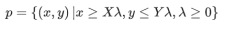
| [34] | Noura, A. A.,. Jahanshahloo, H. F., G. R., Rashidi, S. F. (2011) Super-efficiency in DEA by effectiveness of each unit in society, Applied Mathematics Letters, Volume 24, Issue 5, Pages 623-626, ISSN 0893-9659. |
[34]
where λ is a non-negative vector in Rn.
A study consider an expression for describing a certain
DMU
o= (x
o, y
o) as
| [34] | Noura, A. A.,. Jahanshahloo, H. F., G. R., Rashidi, S. F. (2011) Super-efficiency in DEA by effectiveness of each unit in society, Applied Mathematics Letters, Volume 24, Issue 5, Pages 623-626, ISSN 0893-9659. |
[34]
:
With λ ≥ 0, s− ≥ 0 and s+ ≥ 0. The vector s− ∈ Rm and s+ ∈ Rs indicate the input excess and output shortfall of this expression, respectively, and are called slacks.
From the condition X ≥ 0 and λ ≥0, it holds that
Using s
− and s
+, Noura, Jahanshahloo
| [34] | Noura, A. A.,. Jahanshahloo, H. F., G. R., Rashidi, S. F. (2011) Super-efficiency in DEA by effectiveness of each unit in society, Applied Mathematics Letters, Volume 24, Issue 5, Pages 623-626, ISSN 0893-9659. |
[34]
define an index ρ as follows:
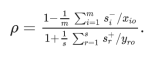
| [34] | Noura, A. A.,. Jahanshahloo, H. F., G. R., Rashidi, S. F. (2011) Super-efficiency in DEA by effectiveness of each unit in society, Applied Mathematics Letters, Volume 24, Issue 5, Pages 623-626, ISSN 0893-9659. |
[34]
It can be verified that ρ satisfies the properties (i) units invariant and (ii) monotone decreasing in input/output slacks.
From (84), it holds that:
0 < ρ ≤1.
In an effort to estimate the efficiency of (xo, yo), they formulate the following fractional program SBM in λ, s− and s+.
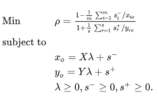
| [34] | Noura, A. A.,. Jahanshahloo, H. F., G. R., Rashidi, S. F. (2011) Super-efficiency in DEA by effectiveness of each unit in society, Applied Mathematics Letters, Volume 24, Issue 5, Pages 623-626, ISSN 0893-9659. |
[34]
SBM can be transformed into a linear program using the Charnes–Cooper transformation in a comparable way to the CCR model.
The analysis of the level 1 and 2 SE ratings is derived from the seven models implemented for DMUs previously assumed to be homogeneous and not arranged in a group structure
| [3] | Muvingi, J., Peer, A. A. I., Hosseinzadeh Lotfi, F., & Ozsoy, V. S. (2023). Hierarchical groups DEA super-efficiency and group TOPSIS technique: Application on mobile money agents’ locations, Expert Systems with Applications, Volume 234, 0957-4174, https://doi.org/10.1016/j.eswa.2023.121033 |
[3]
. To ensure that those models are applicable to the SE evaluation of DMUs in a two-level hierarchical group structure, additional constraints were added:
DSE-1 ratings
| [3] | Muvingi, J., Peer, A. A. I., Hosseinzadeh Lotfi, F., & Ozsoy, V. S. (2023). Hierarchical groups DEA super-efficiency and group TOPSIS technique: Application on mobile money agents’ locations, Expert Systems with Applications, Volume 234, 0957-4174, https://doi.org/10.1016/j.eswa.2023.121033 |
[3]
.
A study introduced an improved Super SBM model that can handle negative data, which is an improvement from the traditional super SBM models. They propose a non-radial SE model capable of ranking efficient DMUs
| [3] | Muvingi, J., Peer, A. A. I., Hosseinzadeh Lotfi, F., & Ozsoy, V. S. (2023). Hierarchical groups DEA super-efficiency and group TOPSIS technique: Application on mobile money agents’ locations, Expert Systems with Applications, Volume 234, 0957-4174, https://doi.org/10.1016/j.eswa.2023.121033 |
[3]
.
Muvingi, Peer
| [3] | Muvingi, J., Peer, A. A. I., Hosseinzadeh Lotfi, F., & Ozsoy, V. S. (2023). Hierarchical groups DEA super-efficiency and group TOPSIS technique: Application on mobile money agents’ locations, Expert Systems with Applications, Volume 234, 0957-4174, https://doi.org/10.1016/j.eswa.2023.121033 |
[3]
consider a modified slacks based SE measure in the presence of negative data. The SE methodology, for example that of Bajec, Tuljak
| [35] | Bajec, P., Tuljak-Suban, D., & Zalokar, E. (2021). A Distance-Based AHP-DEA Super-Efficiency Approach for Selecting an Electric Bike Sharing System Provider: One Step Closer to Sustainability and a Win–Win Effect for All Target Groups. Sustainability, 13(2), 549. https://doi.org/10.3390/su13020549 |
[35]
. is crafted to manage data uncertainties, while the multi-level nature of mobile money agent networks in Muvingi, Peer
| [3] | Muvingi, J., Peer, A. A. I., Hosseinzadeh Lotfi, F., & Ozsoy, V. S. (2023). Hierarchical groups DEA super-efficiency and group TOPSIS technique: Application on mobile money agents’ locations, Expert Systems with Applications, Volume 234, 0957-4174, https://doi.org/10.1016/j.eswa.2023.121033 |
[3]
can be somewhat complex.
The Muvingi, Peer
| [3] | Muvingi, J., Peer, A. A. I., Hosseinzadeh Lotfi, F., & Ozsoy, V. S. (2023). Hierarchical groups DEA super-efficiency and group TOPSIS technique: Application on mobile money agents’ locations, Expert Systems with Applications, Volume 234, 0957-4174, https://doi.org/10.1016/j.eswa.2023.121033 |
[3]
study implemented the TOPSIS method to obtain a clear ranking of all the suburb locations through the incorporation of all the seven DSE ratings
| [3] | Muvingi, J., Peer, A. A. I., Hosseinzadeh Lotfi, F., & Ozsoy, V. S. (2023). Hierarchical groups DEA super-efficiency and group TOPSIS technique: Application on mobile money agents’ locations, Expert Systems with Applications, Volume 234, 0957-4174, https://doi.org/10.1016/j.eswa.2023.121033 |
[3]
. Their ranking results revealed that most of the highly-rated suburb areas are located in low density areas, while the opposite was observed in the TOPSIS ranking of district locations
| [3] | Muvingi, J., Peer, A. A. I., Hosseinzadeh Lotfi, F., & Ozsoy, V. S. (2023). Hierarchical groups DEA super-efficiency and group TOPSIS technique: Application on mobile money agents’ locations, Expert Systems with Applications, Volume 234, 0957-4174, https://doi.org/10.1016/j.eswa.2023.121033 |
[3]
. They conjectured that a complete ranking of the DMUs through TOPSIS was achieved for all district and suburb locations
| [3] | Muvingi, J., Peer, A. A. I., Hosseinzadeh Lotfi, F., & Ozsoy, V. S. (2023). Hierarchical groups DEA super-efficiency and group TOPSIS technique: Application on mobile money agents’ locations, Expert Systems with Applications, Volume 234, 0957-4174, https://doi.org/10.1016/j.eswa.2023.121033 |
[3]
. The adoption of the TOPSIS method provided rankings derived from the ratings of seven diversified SE approaches, which ensured that the merits and demerits of each DEA SE model were considered in the final ranking of DMUs
| [3] | Muvingi, J., Peer, A. A. I., Hosseinzadeh Lotfi, F., & Ozsoy, V. S. (2023). Hierarchical groups DEA super-efficiency and group TOPSIS technique: Application on mobile money agents’ locations, Expert Systems with Applications, Volume 234, 0957-4174, https://doi.org/10.1016/j.eswa.2023.121033 |
[3]
. The TOPSIS method refined the ranking by comparing each agent’s performance against an ideal solution, thereby overcoming the limitations of traditional DEA in distinguishing between efficient units.
Muvingi, Peer
| [3] | Muvingi, J., Peer, A. A. I., Hosseinzadeh Lotfi, F., & Ozsoy, V. S. (2023). Hierarchical groups DEA super-efficiency and group TOPSIS technique: Application on mobile money agents’ locations, Expert Systems with Applications, Volume 234, 0957-4174, https://doi.org/10.1016/j.eswa.2023.121033 |
[3]
used the Principal Component Analysis (PCA) method and the Spearman correlation analysis to verify and validate the TOPSIS results. They found the accuracy of the district location TOPSIS ranking approach to be moderate, at the rate of 61 percent on the observed suburb locations. Mvere
| [6] | Mvere, E. S (2025). A Systematic Review Of The Esmvere Algorithms, Which Are Contributions In The Field Of Uncapacitated Facility Location Problems And K‐Median Problems International Journal of Science Academic Research, Vol. 06 No. 2, 2025, pp. 9352-9362 |
| [23] | Mvere, E. S (2025) An Analysis of the Used Lead Acid Battery (ULAB) Collection Network Mauritius Using the ESMVERE- R-Hamming-k-median Clustering Method., International Journal of Science Academic Research, Vol. 06 No. 1, 2025. |
[6, 23]
used the ESMVERE-R-hamming k-median clustering method to infer opinions of whether there would be a need to introduce a new collection system for ULABs to which 55 percent of the respondents confirmed the need for a new ULAB collection system
| [23] | Mvere, E. S (2025) An Analysis of the Used Lead Acid Battery (ULAB) Collection Network Mauritius Using the ESMVERE- R-Hamming-k-median Clustering Method., International Journal of Science Academic Research, Vol. 06 No. 1, 2025. |
[23]
. However, the study, Muvingi, Peer
| [3] | Muvingi, J., Peer, A. A. I., Hosseinzadeh Lotfi, F., & Ozsoy, V. S. (2023). Hierarchical groups DEA super-efficiency and group TOPSIS technique: Application on mobile money agents’ locations, Expert Systems with Applications, Volume 234, 0957-4174, https://doi.org/10.1016/j.eswa.2023.121033 |
[3]
, contributed to the literature focused on comparing TOPSIS and PCA, as most of the work is on the comparison of DEA and PCA. While Mvere
| [6] | Mvere, E. S (2025). A Systematic Review Of The Esmvere Algorithms, Which Are Contributions In The Field Of Uncapacitated Facility Location Problems And K‐Median Problems International Journal of Science Academic Research, Vol. 06 No. 2, 2025, pp. 9352-9362 |
| [23] | Mvere, E. S (2025) An Analysis of the Used Lead Acid Battery (ULAB) Collection Network Mauritius Using the ESMVERE- R-Hamming-k-median Clustering Method., International Journal of Science Academic Research, Vol. 06 No. 1, 2025. |
[6, 23]
introduced an original, completely new and innovative way of analyzing questionnaire data.
The main contribution of the study Muvingi, Peer
| [3] | Muvingi, J., Peer, A. A. I., Hosseinzadeh Lotfi, F., & Ozsoy, V. S. (2023). Hierarchical groups DEA super-efficiency and group TOPSIS technique: Application on mobile money agents’ locations, Expert Systems with Applications, Volume 234, 0957-4174, https://doi.org/10.1016/j.eswa.2023.121033 |
[3]
includes:
1) It provides insight to bank and Mobile Money Operators (MMOs) regulators into how the characteristics of locations are related to the use of mobile money, represented by MTSU.
2) Regulators can use the efficiency analysis of the locations in the study as a proxy measure for potential financial inclusion in a given location.
3) The study provided a bench-marking analysis of potential MMA locations, allowing banks to strategically locate their branches depending on the influence of MMAs locations on their operations.
4) The location performance results guide MMOs for MMA network scaling.