Stationarity in Prophet Model Forecast: Performance Evaluation Approach

Evelyn Adebola Omotoye; Bunmi Segun Rotimi

doi:doi:10.11648/j.ajtas.20251403.12

Research Article |

| Peer-Reviewed

Stationarity in Prophet Model Forecast: Performance Evaluation Approach

Evelyn Adebola Omotoye

, Bunmi Segun Rotimi^*

Published in American Journal of Theoretical and Applied Statistics (Volume 14, Issue 3)

Received: 29 April 2025 Accepted: 12 May 2025 Published: 30 June 2025

Views: Downloads:

Download PDF

Share This Article

Twitter
Linked In
Facebook

Abstract

Stationarity plays a crucial role in time series analysis, significantly influencing model performance and the reliability of forecasts. Despite its importance, many real-world datasets exhibit non-stationary behaviour, which can lead to misleading or spurious forecasting outcomes. This study explores the impact of stationarity on the performance of the Prophet Model, a scalable time series forecasting tool developed by Facebook, by comparing forecasts from both stationary and non-stationary versions of the same dataset. The monthly international airline passenger data was downloaded from the Kaggle website. We applied the Prophet to generate forecasts from raw (non-stationary) data and its transformed (stationary) version, obtained through first differencing. Three metrics, including the Root Mean Square Error (RMSE), Mean Absolute Error (MAE), and coverage, were used to evaluate both versions of the forecasts. The findings reveal that forecasted values from stationary and non-stationary data exhibit strong correlations with actual values, as confirmed by T-tests and Pearson correlation coefficients. However, the Prophet model demonstrated notably better performance on stationary data compared to the non-stationary version, with the forecast for stationary data showing lower RMSE and MAE values and higher coverage percentages. The study shows the importance of ensuring stationarity before forecasting, even when using advanced models like the Prophet Model. We suggest that integrating stationarity considerations into future iterations of the Prophet algorithm could further enhance its predictive capabilities.

Published in	American Journal of Theoretical and Applied Statistics (Volume 14, Issue 3)
DOI	10.11648/j.ajtas.20251403.12
Page(s)	109-117
Creative Commons	This is an Open Access article, distributed under the terms of the Creative Commons Attribution 4.0 International License (http://creativecommons.org/licenses/by/4.0/), which permits unrestricted use, distribution and reproduction in any medium or format, provided the original work is properly cited.
Copyright	Copyright © The Author(s), 2025. Published by Science Publishing Group

Keywords

Forecasting, RMSE, MAE, Coverage, Prophet, Stationarity, Performance Metrics

1. Introduction

A stationary process has the property that the mean, variance, and autocorrelation structure do not change over time. This stationarity is one common assumption in many time series techniques. Unfortunately, most real-life data are not stationary. The series obtained in real-life occurrences are usually not normally distributed, and the mean and variance may not be constant over a long period. But as proven, non-stationary data are unpredictable and cannot be modelled or forecasted. The results obtained by using non-stationary time series may be spurious as they may indicate a relationship between two variables where one does not exist. To obtain consistent and reliable results, the non-stationary data needs to be made stationary

[1]

. This is a major concern in ensuring that the study data are not subjected to undue generalized modifications under any form of time series model or in the course of any stationarity process because van-Greunen et al., 2014

[2]

posited that the stationarity of a time series can have a significant influence on its properties and forecasting behavior, where the inability to render a time series to the correct form of stationarity can lead to spurious results. Hence, the need to seek the most appropriate time series model with a suitable stationarity method to analyze specific data under study to avoid a significant discrepancy in the forecast.

Essentially, Time-series forecasting has always been a major topic in data science with numerous applications. However, Velicer and Plummer

[3]

noted in their comment on Simonton's study that time series applies to a unique class of problems, can use information about temporal ordering to make statements about causation, and focuses on patterns of change over time; but also suffers from several weaknesses, including problems with generalization from a single study, difficulty in obtaining appropriate measures, and problems with accurately identifying the correct model to represent the data. Adhikari and Agrawal

[4]

gave a general review of some of the most used tools and Petropoulos

[5]

also did a very comprehensive review based on their study. Suitable models in Time series which fit almost perfectly to the various dataset with distinct characteristics, therefore, need logical consideration. Several other time series models have been studied with the focus of identifying the most appropriate prediction methods for different types of situations, away from the usual ARIMA models which are frequently used in econometric analyses. For instance, LSTMs in conjunction with the attention mechanism have been widely used to make predictions in economic and financial time series

[6]

. Machine learning models using LSTMs and CNNs are of widespread use in time-series forecasting, well beyond the ﬁnancial and economic scope.

Currently, one of the latest published forecasting models, called Prophet, is gaining widespread application in time series forecasting across various fields. Taylor and Letham

[7]

developed the Prophet forecasting model for Facebook. Subsequently, they published this model in the same package in R and Python. This allowed the testing of the model by researchers from other research institutes and universities, not least driven by the underlying rationale to develop a modular regression model with interpretive parameters that can be intuitively adjusted by analysts with domain knowledge about the time series (see

[8, 9]

). Prophet model is a procedure for forecasting time series data based on an additive model such as it is assumed that there is no interaction among the various component) where non-linear trends are ﬁt with yearly, weekly, and daily seasonality plus holiday eﬀects

[10]

. The prophet model is especially useful for datasets that: contain an extended period (months or years) of detailed historical observations (hourly daily or weekly); have multiple strong seasonality; Include previously known important but irregular events; have missing data points or large outliers. and have non-linear growth trends that are approaching a limit. Topping et al.

[11]

evaluate Facebook’s Prophet model v0.6 in predicting hourly concentrations of Nitrogen Dioxide [NO₂] over two years across some regions and found that the Prophet model offers a relatively effective and simple way to make predictions about NO₂ at local levels. Lorenzo et al.

[12]

noted that the fundamental dynamics of Prophet are known to be simplicity and scalability; it is speciﬁcally tailored for business forecasting problems and handles missing data very well by construction. On the other, the NN models we construct directly lend themselves to carrying out a multivariate regression, fully exploiting all the collected data; however, they also require some data pre-processing, as does ARIMA. Among other model comparison studies, Chan

[13]

and Yenidoğan

[14]

have compared Prophet to ARIMA models for the prediction of stock prices. Some recent studies on time-series forecasting with Prophet in other relevant areas such as health include an application to COVID-19 outbreak, death, and recovery cases forecasting. Khayyat et al.

[15]

applied the prophet model to covid-19 data in Saudi Arabia to observe and predict the future daily or weekly spread of the pandemic. Their proposed model has a strong ability to forecast the death cases, although its ability to forecast the recovered cases of the COVID-19 dataset is weak and suggests collecting additional data to strengthen the model validation. Luo et al.

[16]

also applied a combined model of SARIMA and Prophet on HIV/AIDS data in Henan and found it appropriate to predict the incidence of disease in that area.

In this study, the strength of the prophet model is assessed based on its performance on non-stationary data and the stationary version. This is an attempt to investigate whether any disparity in the two forecasted results is significant vis-à-vis the real-life data for the period under consideration. To achieve this aim, we specify the methodology in Section 2. Results obtained are presented and discussed in Section 3, and we conclude by recommending that the Prophet Model algorithm should be updated to incorporate the stationarity of the dataset in Section 4.

2. Methodology2.1 The Prophet Model

The prophet model is an open-source library that is based on decomposable models

[10]

. It enables the prediction of time-series data with high accuracy using straightforward parameters. Prophet works with decomposable time series with three main components: Trends, Seasonality, and Holidays. They are combined in the following equation

y (t) = g (t) + s (t) + h (t) + e (t)

(1)

where

y (t)

is the Additive Model,

g (t)

is the Trend Function,

s (t)

is the Seasonality Effect,

h (t)

is the Effects of holidays, and

e (t)

is the Error term. Time (t) is used as the Regressor. The trend Function provides two possible trend models for g(t), which are saturating growth and change points. The Saturating growth model is given by

g (t) = \frac{C}{1 + e^{(- k (t - m))}}

(2)

where

C

is the carrying capacity,

k

is the growth rate,

m

is the offset parameter. Trend change in growth model is incorporated by explicitly defining changepoints where the growth rate is allowed to change. It is given by

g (t) = \frac{C (t)}{1 + e^{(- (k + a {(t)}^{T} δ) (t - (m + a {(t)}^{T} γ))}}

(3)

Where

C (t)

is the carrying capacity over time

t

a {(t)}^{T} δ

is the change in the growth rate over time

t,

γ

Adjust the offset parameter to connect the endpoints of the adjustment.

k

growth rate,

m

is the offset parameter. The seasonality component

s (t)

provides adaptability to the model by allowing periodic changes based on sub-daily, daily, weekly, and yearly seasonality. Prophet relies on the Fourier series to provide an adaptable model of periodic effects.

P

is the regular period of the time series. Seasonal effects are therefore tied to a standard Fourier series;

s (t) = \sum_{n = 1}^{N} (a_{n} \cos \frac{2 πnt}{P} + b_{n} \sin \frac{2 πnt}{P})

(4)

Fitting seasonality requires estimating the 2N parameters

β = [a_{1}, b_{1}, \dots a_{n}, b_{n}]^{T}

. This is done by constructing a matrix of seasonality vectors for each value of t in the historical and future data. This implies that the seasonal component is

s (t) = X (t) β

(5)

N

is the order of the Fourier series,

P

is the period. Also, the impact of a particular holiday on the time series is often similar year after year, making it important to incorporate it into the forecast. The component

h (t)

speaks of predictable events of the year. For each holiday

i,

let

D_{i}

be the set of past and future dates for the holiday. An indicator function represents whether time t is during holiday

i,

and assigns each holiday a parameter.

ki

which is the corresponding change in the forecast. This is done in a similar way as seasonality by generating a matrix of regressors;

Z (t) = [1 (t \in D_{1}), \dots, 1 (t \in D_{L})]

(6)

and taking,

h (t) = Z (t) k

(7)

where

D_{i}

is a set of past and future dates for the holiday,

k

is a vector for the holiday.

2.2. Data Source

In this study, the dataset used was sourced from the internet, corresponding to monthly international airline passengers (in thousands). It is a non-stationary seasonal time series.

2.3. Data Analysis

The data was first tested for stationarity using the augmented Dickey-Fuller (ADF) method

[19]

and was discovered not to be stationary. The Prophet model was applied to the non-stationary data in R to obtain the forecast, then the Mean Absolute Error (MAE), Root Mean Square Error (RMSE), and Coverage were used to determine the performance of the model

[18]

. Thereafter, the first difference of the non-stationary data was taken and tested with ADF, and it was discovered to be stationary at first difference. The Prophet model was applied to the stationary data, the forecast was obtained, and the performance metrics using the Mean Absolute Error (MAE) and Root Mean Square Error (RMSE) were also determined. The validation of the model which compares forecasted values of the prophet model from the Stationary data and the non-stationary data with the actual values using the T-test and the Pearson's correlation coefficient was employed to determine if there is a significant relationship in the Prophet model forecasted values and the actual values from Stationary data and non-stationary data. The performance metrics (MAE, RMSE, and coverage) of the two models were also compared to determine the best model.

2.4. Performance Metrics in the Prophet Model

Three performance metrics used for measuring forecasting accuracy are the Root Mean Square Error (RMSE), the Mean Absolute Error (MAE), and the Coverage.

2.4.1. Root Mean Square Error (RMSE)

RMSE compares forecasted values and observed or known values. The lower the RMSE value, the closer the forecasted and observed values

[17]

. It is given by.

RMSE = \sqrt{\frac{\sum {(y_{hat} - y)}^{2}}{n}}

(8)

where

y_{hat}

is the forecasted value,

y

is the observed value,

n

is the total data points.

2.4.2. Mean Absolute Error (MAE)

MAE measures the average of the absolute error values. The absolute difference between an observed value and a forecasted value is considered when calculating MAE.

MAE = \frac{\sum | y_{hat} - y |}{n}

(9)

where

y_{hat}

is the forecasted value,

y

is the observed value,

n

is the total data points.

2.4.3. Coverage

Coverage gives the percentage probability that the forecasted value will lie between the lower interval (

y_{hat}

lower) and the upper interval (

y_{hat}

upper) predicted by the Prophet Model. A higher coverage value represents lower variability in the dataset

[11]

3. Results and Discussion

3.1. Forecast Obtained from Non-Stationary Data

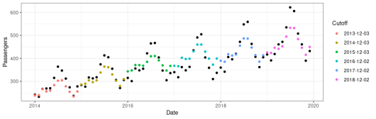
The Prophet Model was applied to the Non-Stationary Data; change points or cutoffs and the error were determined automatically by the model (Figures 1 and 2). The change points were 2013-12-03, 2014-12-03, 2015-12-03, 2016-12-02, 2017-12-02, and 2018-12-02. The change points or cut-off points were periods where the trend of the data was interrupted

[19]

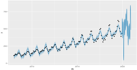
. The model was able to predict the entire 2020 year accurately, with only 12 years of (2008–2019) data. This model is not overfitted due to its ability to predict 2020 effectively (Figure 2).

Download: Download full-size image

Figure 1. Graph showing the Change points of the Airline passenger from 2014 to 2020.

Download: Download full-size image

Figure 2. Prophet Model forecasting for Non-Stationary Data. The Prophet model’s predictions were compared to the actual values. The prediction for the 2020 year is shown.

3.1.1. Performance Metrics from Non-Stationary Data

The performance metrics for non-stationary data using RMSE, MAE, and coverage show that in a 60-day prediction, the MAE value was 20.567, the RMSE value was 25.003, a difference of 4.436, while the coverage was 52% (Table 1). However, predictions were more accurate at the 333-day prediction with an RMSE of 19.425, MAE of 15.319, and a coverage of 64%. The lower the RMSE and MAE, the more accurate the prediction, while the higher the coverage percentage, the more accurate the prediction

[17]

Table 1. Performance Metrics showing the RMSE, MAE, and the Coverage of the model for non-stationary data.

Prediction Days	RMSE	MAE	Coverage
60	25.003	20.567	52%
61	34.190	30.303	33%
88	31.547	25.917	48%
89	25.831	21.416	43%
119	21.620	18.668	29%
120	25.977	22.946	32%
149	24.243	20.925	29%
150	20.741	17.447	50%
180	24.506	21.420	43%
181	29.251	26.124	39%
210	38.801	34.520	29%
211	56.826	52.983	7%
241	56.551	53.853	0%
242	58.030	56.137	0%
272	52.888	49.959	0%
273	32.462	28.329	43%
302	20.295	18.503	57%
303	21.239	18.071	54%
333	19.425	15.319	64%
334	33.003	26.716	36%
363	32.718	26.563	29%
364	35.624	29.245	29%
365	32.660	26.287	43%

y y_{hat}

3.1.2. Comparing the Result of the Actual Values () with the Predicted Values () Using the T-test

Pearson's correlation coefficient of the actual values (y) and the predicted values

(y_{hat})

was 0.919 (Table 2), showing that there is a strong relationship between the actual values and the predicted values. The mean of

y_{hat}

is 374.498 while the mean of

y

is 377.694, which shows that the mean of

y_{hat}

is greater than the mean value of

y

. The sig. value of 0.434 is greater than 0.05, which is the significance level; this implies that there is no significant difference between the actual values and the predicted values for the stationary data.

Table 2. Comparing the result of the actual values (

y

) with the predicted values (

y_{hat}

) for non-stationary data using the T-test.

	Y	$y_{hat}$
Mean	377.694	374.498
Variance	7471.736	5477.117
Pearson Correlation	0.919
Df	71
t Stat	0.787
Sig. Value	0.434

3.2. Forecast Obtained from Stationary Data

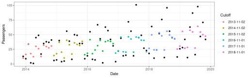
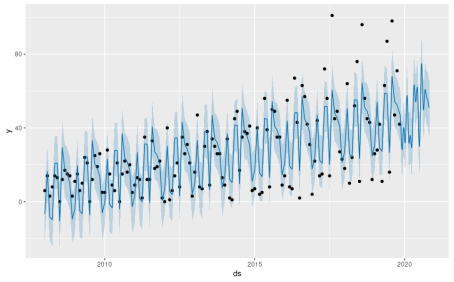
The Data was made stationary by taking the first difference and tested with the Augmented Dickey-Fuller Method (ADF), which gives a sig. value of 0.01, indicating that the data is stationary. The Prophet Model was applied to the Stationary Data; change points or cutoffs, and the error was determined automatically by the model (Figures 3 and 4). The change points were 2013-11-02, 2014-11-02, 2015-11-02, 2016-11-01, 2017-11-01, and 2018-11-01. The change points are observed to differ by one day and one month from the change points obtained for the non-stationary data. This is because there is a loss of a data point when conducting first differencing, hence the difference in the change points by one day and one month. The model was able to predict the entire 2020 year. However, the prediction pattern seems to be slightly different from that of the stationary data (Figure 4).

Download: Download full-size image

Figure 3. Graph showing the Change points of the Stationary Data.

Download: Download full-size image

Figure 4. Prophet Model forecasting for Stationary Data. The Prophet model’s predictions were compared to the actual values. The prediction for 2020 is shown.

3.2.1. Performance Metrics from Stationary Data

The performance metrics for stationary data show that in a 60-day prediction, the MAE value was 8.348, the RMSE value was 9.445, a difference of 1.097, while the coverage was 43% (Table 3). However, predictions were more accurate at the 365-day prediction with an RMSE of 8.213, MAE of 6.472, and a coverage of 68%. Comparing this result with the result obtained from non-stationary data, it is observed that the performance metrics of the stationary data are lower compared to those of the non-stationary data; this indicates that the model of the stationary data is more accurate than that of those obtained from non-stationary data.

Table 3. Performance Metrics showing the RMSE, MAE, and the Coverage of the model for stationary data.

Prediction Days	RMSE	MAE	Coverage
60	9.445	8.348	43%
61	7.687	6.563	62%
91	7.043	5.388	76%
92	13.039	9.267	57%
119	15.148	12.391	33%
120	14.142	13.172	19%
150	11.834	11.197	29%
151	11.461	9.7138	46%
180	12.866	11.221	36%
181	19.186	15.469	36%
211	19.812	15.997	43%
212	20.882	17.434	36%
241	18.445	14.817	36%
242	13.825	11.814	46%
272	11.882	10.557	50%
273	31.098	26.158	21%
303	31.155	26.548	7%
304	18.138	13.395	43%
333	9.657	8.045	57%
334	10.150	7.742	68%
364	9.935	7.695	64%
365	8.214	6.472	68%

3.2.2. Comparing the Result of the Actual Values (y) with the Predicted Values (yhat) from Stationary Data Using the T-test

Pearson's correlation coefficient of the actual values (y) and the predicted values (yhat) was 0.837 (Table 2), showing that there is a strong relationship between the actual values and the predicted values for the stationary data. The sig. value of 0.123 is greater than 0.05, which is the significance level; this implies that there is no significant difference in the actual values and the predicted values for the stationary data.

Table 4. Comparing the result of the actual values (y) with the predicted values (yhat) for stationary data using the T-test.

	Y	Yhat
Mean	35.792	32.921
Variance	622.393	176.819
Pearson Correlation	0.837
Df	71
t Stat	1.561
Sig. value	0.123

3.3. Comparing the Performance Metric of the Prophet Model for Non-Stationary Data and Stationary Data

The result of the average of the RMSE, MAE, and Coverage for both non-Stationary and Stationary data was compared. The RMSE, MAE, and the Coverage of the Non-Stationary Data are 32.758, 28.792, and 34% respectively, while those of Stationary data are 14.775, 12.246, and 44% respectively. This result shows that the Prophet model from the Stationary Data performs better compared to the Prophet model from non-Stationary data.

Table 5. Comparing the Performance Metric of the Prophet model for Non-Stationary Data and Stationary Data.

	RMSE	MAE	Coverage
Non-Stationary	32.758	28.792	34%
Stationary	14.775	12.246	44%

4. Conclusion

The predicted values obtained from both non-stationary data and stationary data are not significantly different from their respective actual values and also indicate strong correlation coefficients. The change points of non-stationary data differ by one day and one month from the change points of stationary data. This arises due to the loss of a data point when conducting the first differencing. However, Performance Metrics results from RMSE, MAE, and coverage indicate that the Prophet model performs better with Stationary data. Like other Times series models which assume stationarity of the dataset, the developers of the Prophet Forecasting model could also consider the stationarity of the dataset in a future update of the Prophet Model algorithm. This may better enhance the performance of the model.

Abbreviations

ADF	Augmented Dickey-Fuller
MSE	Mean Square Error
MAE	Mean Absolute Error
RMSE	Root Mean Square Error
Sig.value	Significant Value

Conflicts of Interest

The authors declare that they have no known conflicts of interest or personal relationships that could have appeared to influence the work reported in this paper.

Appendix

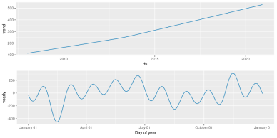
Prophet Model Component Plot for Non-Stationary Data.

Download: Download full-size image

Figure 5. Trend Line and Seasonal variation of the Non-Stationary Data.

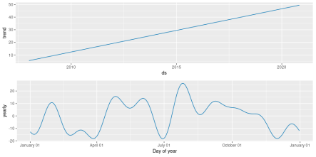
Prophet Model Component Plot for Stationary Data.

Download: Download full-size image

Figure 6. Trend Line and Seasonal variation of the Stationary Data.

References

[1]	Gujarati, D. N. (2006). Essentials of Econometrics. 3rd Edition, McGraw-Hill.
[2]	van Greunen, J., Heymans, A., van Heerden, C., & van Vuuren, G. (2014). The Prominence of Stationarity in Time Series Forecasting. Studies in Economics and Econometrics, 38(1), 1-16. https://doi.org/10.1080/10800379.2014.12097260
[3]	Velicer, W. F., & Plummer, B. A. (1998). Time series analysis in historiometry: a comment on Simonton. Journal of Personality, 66(3), 477–493. https://doi.org/10.1111/1467-6494.00020
[4]	Adhikari, R., & Agrawal, R. K. (2013). An Introductory Study on Time Series Modeling and Forecasting. ArXiv, abs/1302.6613.
[5]	Petropoulos, F., Apiletti, D., Assimakopoulos, V., Babai, M. Z., Barrow, D. K., Taieb, S. B., … Florian Ziel (2021). Forecasting: Theory and practice. arXiv 2021, arXiv: 2012.03854.
[6]	Qiu, J., Wang, B., & Zhou, C. (2020). Forecasting stock prices with long-short term memory neural network based on attention mechanism. PLOS ONE, 15(1), e0227222. https://doi.org/10.1371/journal.pone.0227222
[7]	Taylor, S. J., & Letham, B. (2017). Forecasting at Scale. The American Statistician, 72(1), 37-45. https://doi.org/10.1080/00031305.2017.1380080
[8]	Makridakis, S., Spiliotis, E., and Assimakopoulos, V. (2018). Statistical and Machine Learning forecasting methods: Concerns and ways forward. PLOS ONE, 13(3), e0194889. https://doi.org/10.1371/journal.pone.0194889
[9]	Žunić, E., Korjenić, K., Hodžić, K., & Đonko, D. (2020). Application of Facebook’s Prophet Algorithm for Successful Sales Forecasting Based on Real-world Data. International Journal of Computer Science and Information Technology, 12(2), 23–36. https://doi.org/10.5121/ijcsit.2020.12203
[10]	Topping, D., Watts, D., Coe, H., Evans, J., Bannan, T. J., Lowe, D., Jay, C., and Taylor, J. W. (2020). Evaluating the use of Facebook's Prophet model v0.6 in forecasting concentrations of NO₂ at single sites across the UK and in response to the COVID-19 lockdown in Manchester, England. Geosci. Model Dev. Discuss. [preprint], https://doi.org/10.5194/gmd-2020-270 2020
[11]	Menculini, L., Marini, A., Proietti, M., Garinei, A., Bozza, A., Moretti, C., & Marconi, M. (2021). Comparing Prophet and Deep Learning to ARIMA in Forecasting Wholesale Food Prices. Forecasting, 3(3), 1-19.
[12]	Chan, W. N. (2020). Time-Series Data Mining: Comparative Study of ARIMA and Prophet Methods for Forecasting Closing Prices of Myanmar Stock Exchange. J. Comput. Appl. Res., 1, 75–80.
[13]	Yenidoğan, I., Çayir, A., Kozan, O., Dağ, T., & Arslan, Ç. (2018). Bitcoin Forecasting Using ARIMA and PROPHET. 2018 3rd International Conference on Computer Science and Engineering (UBMK), 621-624.
[14]	Khayyat, M., Laabidi, K., Almalki, N., & Al-zahrani, M. (2021). Time Series Facebook Prophet Model and Python for COVID-19 Outbreak Prediction. Computers, Materials & Continua. https://doi.org/10.32604/cmc.2021.014918
[15]	Luo, Z., Jia, X., Bao, J., Song, Z., Zhu, H., Liu, M., Yang, Y., & Shi, X. (2022). A Combined Model of SARIMA and Prophet Models in Forecasting AIDS Incidence in Henan Province, China. Int. J. Environ. Res. Public Health, 19, 5910. https://doi.org/10.3390/ijerph19105910
[16]	Lendave, V. (2021). A Guide to Different Evaluation Metrics for Time Series Forecasting Models. Retrieved from https://analyticsindiamag.com/a-guide-to-different-evaluation-metrics-for-time-series-forecasting-models/
[17]	Wang, W., & Lu, Y. (2018). Analysis of the Mean Absolute Error (MAE) and the Root Mean Square Error (RMSE) in Assessing Rounding Model. IOP Conference Series: Materials Science and Engineering, 324, 012049. https://doi.org/10.1088/1757-899x/324/1/012049
[18]	Cheung, Y. W., & Lai, K. S. (1995). Lag order and critical values of the augmented Dickey-Fuller test. Journal of Business & Economic Statistics, 13(3), 277–280.
[19]	Vishwas, B. V., & Patel, A. (2020). Prophet. In: Hands-on Time Series Analysis with Python. Apress, Berkeley, CA. https://doi.org/10.1007/978-1-4842-5992-4_8

Cite This Article

Plain Text BibTeX RIS

APA Style

Omotoye, E. A., Rotimi, B. S. (2025). Stationarity in Prophet Model Forecast: Performance Evaluation Approach. American Journal of Theoretical and Applied Statistics, 14(3), 109-117. https://doi.org/10.11648/j.ajtas.20251403.12

Copy | Download

ACS Style

Omotoye, E. A.; Rotimi, B. S. Stationarity in Prophet Model Forecast: Performance Evaluation Approach. Am. J. Theor. Appl. Stat. 2025, 14(3), 109-117. doi: 10.11648/j.ajtas.20251403.12

Copy | Download

AMA Style

Omotoye EA, Rotimi BS. Stationarity in Prophet Model Forecast: Performance Evaluation Approach. Am J Theor Appl Stat. 2025;14(3):109-117. doi: 10.11648/j.ajtas.20251403.12

Copy | Download

@article{10.11648/j.ajtas.20251403.12,
  author = {Evelyn Adebola Omotoye and Bunmi Segun Rotimi},
  title = {Stationarity in Prophet Model Forecast: Performance Evaluation Approach
},
  journal = {American Journal of Theoretical and Applied Statistics},
  volume = {14},
  number = {3},
  pages = {109-117},
  doi = {10.11648/j.ajtas.20251403.12},
  url = {https://doi.org/10.11648/j.ajtas.20251403.12},
  eprint = {https://article.sciencepublishinggroup.com/pdf/10.11648.j.ajtas.20251403.12},
  abstract = {Stationarity plays a crucial role in time series analysis, significantly influencing model performance and the reliability of forecasts. Despite its importance, many real-world datasets exhibit non-stationary behaviour, which can lead to misleading or spurious forecasting outcomes. This study explores the impact of stationarity on the performance of the Prophet Model, a scalable time series forecasting tool developed by Facebook, by comparing forecasts from both stationary and non-stationary versions of the same dataset. The monthly international airline passenger data was downloaded from the Kaggle website. We applied the Prophet to generate forecasts from raw (non-stationary) data and its transformed (stationary) version, obtained through first differencing. Three metrics, including the Root Mean Square Error (RMSE), Mean Absolute Error (MAE), and coverage, were used to evaluate both versions of the forecasts. The findings reveal that forecasted values from stationary and non-stationary data exhibit strong correlations with actual values, as confirmed by T-tests and Pearson correlation coefficients. However, the Prophet model demonstrated notably better performance on stationary data compared to the non-stationary version, with the forecast for stationary data showing lower RMSE and MAE values and higher coverage percentages. The study shows the importance of ensuring stationarity before forecasting, even when using advanced models like the Prophet Model. We suggest that integrating stationarity considerations into future iterations of the Prophet algorithm could further enhance its predictive capabilities.
},
 year = {2025}
}

Copy | Download

TY  - JOUR
T1  - Stationarity in Prophet Model Forecast: Performance Evaluation Approach

AU  - Evelyn Adebola Omotoye
AU  - Bunmi Segun Rotimi
Y1  - 2025/06/30
PY  - 2025
N1  - https://doi.org/10.11648/j.ajtas.20251403.12
DO  - 10.11648/j.ajtas.20251403.12
T2  - American Journal of Theoretical and Applied Statistics
JF  - American Journal of Theoretical and Applied Statistics
JO  - American Journal of Theoretical and Applied Statistics
SP  - 109
EP  - 117
PB  - Science Publishing Group
SN  - 2326-9006
UR  - https://doi.org/10.11648/j.ajtas.20251403.12
AB  - Stationarity plays a crucial role in time series analysis, significantly influencing model performance and the reliability of forecasts. Despite its importance, many real-world datasets exhibit non-stationary behaviour, which can lead to misleading or spurious forecasting outcomes. This study explores the impact of stationarity on the performance of the Prophet Model, a scalable time series forecasting tool developed by Facebook, by comparing forecasts from both stationary and non-stationary versions of the same dataset. The monthly international airline passenger data was downloaded from the Kaggle website. We applied the Prophet to generate forecasts from raw (non-stationary) data and its transformed (stationary) version, obtained through first differencing. Three metrics, including the Root Mean Square Error (RMSE), Mean Absolute Error (MAE), and coverage, were used to evaluate both versions of the forecasts. The findings reveal that forecasted values from stationary and non-stationary data exhibit strong correlations with actual values, as confirmed by T-tests and Pearson correlation coefficients. However, the Prophet model demonstrated notably better performance on stationary data compared to the non-stationary version, with the forecast for stationary data showing lower RMSE and MAE values and higher coverage percentages. The study shows the importance of ensuring stationarity before forecasting, even when using advanced models like the Prophet Model. We suggest that integrating stationarity considerations into future iterations of the Prophet algorithm could further enhance its predictive capabilities.

VL  - 14
IS  - 3
ER  -

Copy | Download

Author Information

Evelyn Adebola Omotoye

Department of Mathematical Sciences, Adekunle Ajasin University, Akungba Akoko, Ondo State, Nigeria

Contact Email

http://orcid.org/0000-0003-3945-4432
Bunmi Segun Rotimi

Department of Mathematical Sciences, Adekunle Ajasin University, Akungba Akoko, Ondo State, Nigeria

Contact Email

http://orcid.org/0009-0001-1703-2960

Download PDF

Plain Text BibTeX RIS

APA Style

Omotoye, E. A., Rotimi, B. S. (2025). Stationarity in Prophet Model Forecast: Performance Evaluation Approach. American Journal of Theoretical and Applied Statistics, 14(3), 109-117. https://doi.org/10.11648/j.ajtas.20251403.12

Copy | Download

ACS Style

Omotoye, E. A.; Rotimi, B. S. Stationarity in Prophet Model Forecast: Performance Evaluation Approach. Am. J. Theor. Appl. Stat. 2025, 14(3), 109-117. doi: 10.11648/j.ajtas.20251403.12

Copy | Download

AMA Style

Omotoye EA, Rotimi BS. Stationarity in Prophet Model Forecast: Performance Evaluation Approach. Am J Theor Appl Stat. 2025;14(3):109-117. doi: 10.11648/j.ajtas.20251403.12

Copy | Download

@article{10.11648/j.ajtas.20251403.12,
  author = {Evelyn Adebola Omotoye and Bunmi Segun Rotimi},
  title = {Stationarity in Prophet Model Forecast: Performance Evaluation Approach
},
  journal = {American Journal of Theoretical and Applied Statistics},
  volume = {14},
  number = {3},
  pages = {109-117},
  doi = {10.11648/j.ajtas.20251403.12},
  url = {https://doi.org/10.11648/j.ajtas.20251403.12},
  eprint = {https://article.sciencepublishinggroup.com/pdf/10.11648.j.ajtas.20251403.12},
  abstract = {Stationarity plays a crucial role in time series analysis, significantly influencing model performance and the reliability of forecasts. Despite its importance, many real-world datasets exhibit non-stationary behaviour, which can lead to misleading or spurious forecasting outcomes. This study explores the impact of stationarity on the performance of the Prophet Model, a scalable time series forecasting tool developed by Facebook, by comparing forecasts from both stationary and non-stationary versions of the same dataset. The monthly international airline passenger data was downloaded from the Kaggle website. We applied the Prophet to generate forecasts from raw (non-stationary) data and its transformed (stationary) version, obtained through first differencing. Three metrics, including the Root Mean Square Error (RMSE), Mean Absolute Error (MAE), and coverage, were used to evaluate both versions of the forecasts. The findings reveal that forecasted values from stationary and non-stationary data exhibit strong correlations with actual values, as confirmed by T-tests and Pearson correlation coefficients. However, the Prophet model demonstrated notably better performance on stationary data compared to the non-stationary version, with the forecast for stationary data showing lower RMSE and MAE values and higher coverage percentages. The study shows the importance of ensuring stationarity before forecasting, even when using advanced models like the Prophet Model. We suggest that integrating stationarity considerations into future iterations of the Prophet algorithm could further enhance its predictive capabilities.
},
 year = {2025}
}

Copy | Download

TY  - JOUR
T1  - Stationarity in Prophet Model Forecast: Performance Evaluation Approach

AU  - Evelyn Adebola Omotoye
AU  - Bunmi Segun Rotimi
Y1  - 2025/06/30
PY  - 2025
N1  - https://doi.org/10.11648/j.ajtas.20251403.12
DO  - 10.11648/j.ajtas.20251403.12
T2  - American Journal of Theoretical and Applied Statistics
JF  - American Journal of Theoretical and Applied Statistics
JO  - American Journal of Theoretical and Applied Statistics
SP  - 109
EP  - 117
PB  - Science Publishing Group
SN  - 2326-9006
UR  - https://doi.org/10.11648/j.ajtas.20251403.12
AB  - Stationarity plays a crucial role in time series analysis, significantly influencing model performance and the reliability of forecasts. Despite its importance, many real-world datasets exhibit non-stationary behaviour, which can lead to misleading or spurious forecasting outcomes. This study explores the impact of stationarity on the performance of the Prophet Model, a scalable time series forecasting tool developed by Facebook, by comparing forecasts from both stationary and non-stationary versions of the same dataset. The monthly international airline passenger data was downloaded from the Kaggle website. We applied the Prophet to generate forecasts from raw (non-stationary) data and its transformed (stationary) version, obtained through first differencing. Three metrics, including the Root Mean Square Error (RMSE), Mean Absolute Error (MAE), and coverage, were used to evaluate both versions of the forecasts. The findings reveal that forecasted values from stationary and non-stationary data exhibit strong correlations with actual values, as confirmed by T-tests and Pearson correlation coefficients. However, the Prophet model demonstrated notably better performance on stationary data compared to the non-stationary version, with the forecast for stationary data showing lower RMSE and MAE values and higher coverage percentages. The study shows the importance of ensuring stationarity before forecasting, even when using advanced models like the Prophet Model. We suggest that integrating stationarity considerations into future iterations of the Prophet algorithm could further enhance its predictive capabilities.

VL  - 14
IS  - 3
ER  -

Copy | Download