Weibull Distribution and Approximation, by the Finite Volume Method, of the Ultim Ruin Probability Constructed from the Hawkes Variable Memory Process

Souleymane Badini; Frédéric Bere

doi:doi:10.11648/j.ajtas.20251404.11

Research Article |

| Peer-Reviewed

Weibull Distribution and Approximation, by the Finite Volume Method, of the Ultim Ruin Probability Constructed from the Hawkes Variable Memory Process

Souleymane Badini^*

, Frédéric Bere

Published in American Journal of Theoretical and Applied Statistics (Volume 14, Issue 4)

Received: 31 May 2025 Accepted: 16 June 2025 Published: 4 July 2025

Views: Downloads:

Download PDF

Share This Article

Twitter
Linked In
Facebook

Abstract

It measures the risk that a system or company fails to maintain its elf over time. In this article, we provide an approximation of the probability of ruin at the infinite horizon whose inter-arrivals of claims follow the Hawks process and the amount of claims follows the Weibull distribution, with independence between these two processes. Using the Finite Volume Method is a numerical approach for solving partial differential equations. It consists of dividing the computational domain into discrete volumes and applying local approximations to obtain a global solution. This method can be used to estimate complex probabilities., a stochastic model with variable memory, it is possible to capture the temporal dependence of events. This allows us to analyze situations where the past directly influences the probability of occurrence of future events. This approximation is done using the finite volume method, which is a numerical approach for solving partial differential equations. It consists of dividing the computational domain into discrete volumes and applying local approximations to obtain a global solution. This method can be used to estimate complex probabilities. This is the case in our work; which consists of solving a second-order integro-differential equation, two cases of which are considered on the Weibull parameter η: if η=1, then the distribution of claim amounts is exponential. On the other hand, if η≥2, then the results lead us to a system of linear equations for which we use the finite volume method to obtain a numerical solution.

Published in	American Journal of Theoretical and Applied Statistics (Volume 14, Issue 4)
DOI	10.11648/j.ajtas.20251404.11
Page(s)	118-125
Creative Commons	This is an Open Access article, distributed under the terms of the Creative Commons Attribution 4.0 International License (http://creativecommons.org/licenses/by/4.0/), which permits unrestricted use, distribution and reproduction in any medium or format, provided the original work is properly cited.
Copyright	Copyright © The Author(s), 2025. Published by Science Publishing Group

Keywords

Finite Volume Method, Integro-differential Equation, Probability of Ruin, The Finite Volume Method

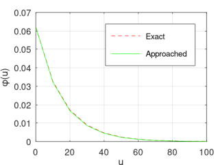
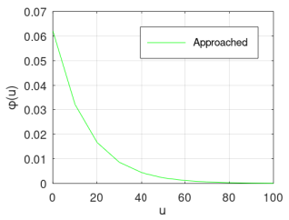
1. Introduction

In insurance, failure theory aims to mathematically analyze random fluctuations in insurance company calculations.

The Weibull distribution is a probability distribution widely used in reliability and statistical analysis due to its ability to model a variety of behaviors related to system failure times. Its flexibility lies in its parameters, which allow the shape and scale to be adapted to describe different practical situations.

Approximating complex phenomena, such as the ultimate failure probability, using the finite volume method is a powerful approach in numerical analysis. By subdividing a domain into finite elements, this method allows complex equations to be solved approximately and efficiently.

When we discuss stochastic processes with variable memory, such as the Hawkes process, we are dealing with dynamic systems where past events influence future probabilities. This framework is particularly relevant for the study of ultimate failure, allowing us to capture temporal dependencies and interactions between events.

This topic combines statistical techniques, numerical methods, and stochastic models to analyze and predict critical events in diverse contexts, ranging from insurance to complex systems.

The risk model of particular interest here is the probability of failure at an infinite horizon. In this article, we seek to determine a finite volume approximation of the ultimate failure probability of the risk model considered in the study of

[1]

. This risk model uses the Hawkes process as the law of inter-arrivals of claims, except that here we will use the Weibull distribution as the law of claims amounts which we define in section (2). We will carry out this work using the numerical methods described in the study of

[3-7]

. Among these methods, we find the finite volume method which will allow us to solve the second-order integral-differential equation that we will derive from the following integral-differential equation:

\frac{\partial}{\partial u} φ (u) = \frac{δ}{c} φ (u) + \frac{λγ}{2 πc} [e^{\frac{δ}{c} u} \int_{0}^{+ \infty} e^{- \frac{δ}{c} y} ϕ (y - u) σ (y) d - \int_{0}^{u} ϕ (y - u) σ (y) dy - (1 + \frac{αλ (2 β - α)}{(β - α) ²})]

(1)

with

ϕ (y - u) = \frac{- αλ (2 β - α) \times 2 \times (- (1 / c)) (((y - u) / c))}{[(β - α) ² + (((y - u) / c)) ²] ²}

And

σ (y) = \int_{0}^{y} ν (y - x) e^{- γx} dx + \int_{y}^{+ \infty} w (y, x - y) e^{- γx} dx

one of the results given in the study of

[1]

. In order to carry out our work successfully, we also draw inspiration from the work done in the study of

[8-14]

. Then we will give the results obtained in the context of this article, in particular the result of the numerical resolution in the case

η = 1

and that of

η \geq 2

We will certainly end with a conclusion in which we will give the limits and advantages of this approach to finite volumes and also perspectives.

2. Preliminaries

The reserve model R(t) that we use in this article is:

R (t) = u + ct - \sum_{i = 1}^{N (t)} X_{i}

(2)

In this reserve model, N(t) is a counting process with variable memory which represents the number of claims at time

t > 0

. The inter-arrivals follow a Hawkes process in the study of

[2]

. Whose ruin time

τ

is defined by:

τ = \inf {t \geq 0; R (t) < 0}

The ultimate probability of ruin is therefore defined by:

φ (u) = P (τ < \infty | R (0) = u)

φ (u)

is the solution to the equation (1) with

\lim_{u \to + \infty} φ (u) = 0

The Laplace transform of

φ

using the equation (1) is defined as follows:

L_{φ (s)} = \frac{[(cϕ (0) + Hϕ (z) + (H / β)) (s ² + βs) - As - Aβ - Ks ²] [γ + s]}{cs ² (s + β) [(Q + 1) s + γ]}

(3)

with A, H, K and Q constants defined by:

A = \frac{λγ}{2 π} (1 + \frac{α λ (2 β - α)}{{(β - α)}^{2}}); H = \frac{λ^{2} c^{2} γα (2 β - α)}{2 π}

K = \frac{λ ² cγ ² α (2 β - α)}{2 π (β - α)}; Q = \frac{λ ² c ² γα (2 β - α)}{2 π (β - α)}

For more details (in the study of

[1]

We also wish to recall that the sequences of variables

{(X_{i})}_{i \geq 1}

represent the amounts of claims which are independent and identically distributed according to the Weibull law. The Weibull distribution is a continuous random variable that is often used to analyze lifetime data, failure time model, and access reliability in the study of

[15]

. This distribution was first introduced by Wallodi Weibull in 1951 and has been widely used in reliability engineering, survival analysis, and other fields. It is often applied in insurance companies to model loss distribution due to its flexibility. The probability density function

f_{X}

of the Weibull random variable is:

f_{X} (x, γ, η) = ηγ {(γx)}^{η - 1} e^{- {(γx)}^{η}}

(4)

with

η > 0

and

γ > 0

the parameters. When

η = 1

, the Weibull distribution becomes an exponential distribution with parameter

γ

and probability density

f_{X}

defined by:

f_{X} (x, γ, η) = γ e^{- γx}

(5)

In the following, we will discuss the probability of ruin at the infinite horizon according to the Weibull distribution is divided according to the parameter η. When the parameter

η = 1

, the probability of ruin can be determined analytically using the Laplace transform method (3). However, when

η \geq 2

, the Laplace transform method can no longer be used because of a step that requires the calculation of an improper integral that cannot be solved analytically. To overcome this challenge (case

η \geq 2

), we will use the finite difference method to solve the equation.

3. Results

In this section, we first treat the case

η = 1

and secondly the case

η \geq 2

using the finite volume method.

3.1. Case η=1

Theorem 3.1: The probability of ruin at the infinite horizon

φ (u)

is defined as follows for all

u \geq 0

Mφ = X

(6)

with

M = (\begin{matrix} \begin{matrix} 1 & 0 & 0 \\ \frac{c - δ}{Δu} & \frac{δ - 2 c}{Δu} + δ & \frac{c}{Δu} \\ 0 & ⋱ & ⋱ \end{matrix} & \begin{matrix} \dots & 0 & 0 \\ 0 & \dots & 0 \\ ⋱ & ⋱ & ⋮ \end{matrix} \\ \begin{matrix} ⋮ & ⋱ & ⋱ \\ 0 & \dots & 0 \\ 0 & \dots & \dots \end{matrix} & \begin{matrix} ⋱ & ⋱ & 0 \\ \frac{c - δ}{Δu} & \frac{δ - 2 c}{Δu} + δ & \frac{c}{Δu} \\ \dots & \dots & 1 \end{matrix} \end{matrix})

φ = (\begin{matrix} φ (u ₀) \\ φ (u ₁) \\ φ (u ₂) \\ ⋮ \\ φ (u_{i}) \\ ⋮ \\ φ (u_{N - 1}) \\ φ (u_{N}) \end{matrix})

X = (\begin{matrix} (\frac{β θ_{1} - θ_{2}}{c (R + β)}) e^{- βu} + (\frac{R θ_{1} - θ_{2}}{c (R + β)}) e^{Ru} \\ g (u_{1}) \\ g (u_{2}) \\ ⋮ \\ g (u_{i}) \\ ⋮ \\ g (u_{N - 1}) \\ g (u_{N}) \end{matrix})

g (u_{i}) = (\frac{α λ^{2} (2 β - α) ((\frac{1}{c^{2}})) [1 + 4 {(\frac{u_{i}}{c})}^{2}] u_{i}}{2 π (u_{i} + β) {[{(β - α)}^{2} + {(\frac{u_{i}}{c})}^{2}]}^{3}}) (1 - e^{- (\frac{δ u_{i}}{c})})

Lemma 3.1: The probability of ruin at the infinite horizon

φ (u)

satisfies the following integro-differential equation:

c \frac{\partial ²}{\partial u ²} φ (u) - δ \frac{\partial}{\partial u} φ (u) + δ φ (u) = \frac{λγ}{2 π} [\int_{0}^{u} ψ (u - y) σ (y) dy - \int_{0}^{u} ϕ (u - y) σ (y) dy]

(7)

With

ψ (u - y) = e^{- δ (\frac{u - y}{c})} \frac{\partial}{\partial u} ϕ (y - u)

and

\frac{\partial}{\partial u} ϕ (y - u) = \frac{- 2 αλ (2 β - α) ((\frac{1}{c^{2}})) [1 + 4 {(\frac{u_{i}}{c})}^{2}]}{{[{(β - α)}^{2} + {(\frac{u_{i}}{c})}^{2}]}^{3}}

Proof.

Using the equation (3) with

σ (y) = \int_{0}^{y} ν (y - x) e^{- γx} dx + \int_{y}^{+ \infty} w (y, x - y) e^{- γx} dx

Confer in the study of

[1]

. We now determine the second derivative of

φ (u)

. Using the equation (1)

\frac{\partial^{2}}{\partial u^{2}} φ (u) = \frac{δ}{c} \frac{\partial}{\partial u} φ (u) + \frac{λγ}{2 π} [\frac{\partial}{\partial u} (\int_{u}^{+ \infty} e^{- δ (\frac{u - y}{c})} ϕ (y - u) σ (y) dy - \int_{0}^{u} ϕ (u - y) σ (y) dy)]

= \frac{δ}{c} \frac{\partial}{\partial u} φ (u) + \frac{λγ}{2 π} [\frac{\partial}{\partial u} (\int_{u}^{+ \infty} e^{- δ (\frac{u - y}{c})} ϕ (y - u) σ (y) dy) - e^{- δ \times 0} ϕ (0) - \int_{0}^{u} \frac{\partial}{\partial u} (ϕ (u - y) σ (y)) dy + ϕ (0)]

= \frac{δ}{c} \frac{\partial}{\partial u} φ (u) - \frac{δ}{c} φ (u) + \frac{λγ}{2 π} + [\int_{0}^{+ \infty} e^{- δ (\frac{u - y}{c})} \frac{\partial}{\partial u} ϕ (y - u) σ (y) dy - \int_{0}^{u} \frac{\partial}{\partial u} (ϕ (u - y) σ (y)) dy]

So this gives us:

c \frac{\partial^{2}}{\partial u^{2}} φ (u) - δ \frac{\partial}{\partial u} φ (u) + δ φ (u) = \frac{λγ}{2 π} [\int_{0}^{+ \infty} e^{- δ (\frac{u - y}{c})} \frac{\partial}{\partial u} ϕ (y - u) σ (y) dy - \int_{0}^{u} \frac{\partial}{\partial u} (ϕ (u - y) σ (y)) dy]

We work at the infinite horizon so

0 \leq u < + \infty

and by setting:

ψ (u - y) = e^{- δ (\frac{u - y}{c})} \frac{\partial}{\partial u} ϕ (y - u) .

we get:

c \frac{\partial^{2}}{\partial u^{2}} φ (u) - δ \frac{\partial}{\partial u} φ (u) + δ φ (u) = \frac{λγ}{2 π} [\int_{0}^{u} ψ (u - y) σ (y) dy - \int_{0}^{u} ϕ (u - y) σ (y) dy]

Due to the complexity of the analytical solution of the equation (7) in the case where ϕ(u) is the probability of ruin at the infinite horizon, we propose a numerical approach for the solution. The finite volume method allows the solution of the equation (7) (approximation), this is given by the following lemma:

Lemma 3.2: Pour

0 \leq u < + \infty

et i allant de 1 à

N - 1

nous For

0 \leq u < + \infty

and i ranging from 1 to

N - 1

we:

[\frac{c - δ}{Δu}] φ (u_{i + 1}) + [\frac{δ - 2 c}{Δu} + δ] φ (u_{i}) + [\frac{c}{Δu}] φ (u_{i - 1}) =

\frac{λγ u_{i}}{4 π} [ψ (u_{i}) σ (0) + ψ (0) σ (u_{i}) - \frac{\partial}{\partial u_{i}} χ (u_{i}) σ (0) - \frac{\partial}{\partial u} χ (0) σ (u_{i})]

(8)

Proof.

Here we use the finite volume method to prove the equation (8). Let the partition of the interval

u \in [0; L]

be defined as follows:

u ₀ = 0 < u ₁ < u ₂ < \dots < u_{N} = L

with L the size and

Δu = \frac{L}{N}

the step or discretization such that

u_{i} = iΔu, n = 0; 1; \dots; N

. The first and second derivatives of the equation (7) can be approximated by the first and second order finite volume method, this gives us:

\frac{\partial}{\partial u} φ (u) \approx \frac{φ_{E} (u) - φ_{P} (u)}{Δu}

(9)

\frac{\partial ²}{\partial u ²} φ (u) \approx \frac{φ_{E} (u) - φ_{P} (u)}{Δu} - \frac{φ_{P} (u) - φ_{W} (u)}{Δu} = \frac{φ_{E} (u) - 2 φ_{P} (u) + φ_{W} (u)}{Δu}

(10)

Let’s ask

φ_{P} (u) = φ (u_{i})

φ_{E} (u) = φ (u_{i + 1})

and

φ_{W} (u) = φ (u_{i - 1})

, the equalities (9) and (10) are transformed into:

\frac{\partial}{\partial u} φ (u_{i}) \approx \frac{φ (u_{i + 1}) - φ (u_{i})}{Δu}

(11)

\frac{\partial ²}{\partial u ²} φ (u_{i}) \approx \frac{φ (u_{i + 1}) - 2 φ (u_{i}) + φ (u_{i - 1})}{Δu}

(12)

The set of points

M_{i} (u_{i} φ (u_{i}),)

are solutions of the equation (8). They describe the trajectory of the solutions given by Figures 1 and 2. Also using the trapezoid method, we obtain the approximations of the integrals of the second member of the equation (7) which gives:

\int_{0}^{u_{i}} ψ (u_{i} - y) σ (y) dy \approx \frac{u_{i}}{2} [ψ (u_{i}) σ (0) + ψ (0) σ (u_{i})]

(13)

\int_{0}^{u_{i}} \frac{\partial}{\partial u_{i}} ϕ (u_{i} - y) σ (y) dy \approx \frac{u_{i}}{2} [\frac{\partial}{\partial u_{i}} ϕ (u_{i}) σ (0) + \frac{\partial}{\partial u_{i}} ϕ (0) σ (u_{i})]

(14)

The equations (7), (11), (12), (13) and (14) gives the equation (8) for i ranging from 1 to

N - 1

Now we have the necessary elements for the proof of the theorem.

Proof of Theorem 3.1:

The equation (3) which represents the Laplace transform of

φ (u)

allows us to obtain the following expression (for more details in the study of

[1]

φ (u) = \frac{β θ_{1} - θ_{2}}{c (R + β)} e^{- βu} + \frac{R θ_{1} + θ_{2}}{c (R + β)} e^{Ru}

(15)

With

R = \frac{- γ}{Q + 1} < 0

The equation (15) implies that:

\lim_{u \to + \infty} φ (u) = 0

(16)

Using equalities of Lemma 3.1, we obtain the following equations:

ψ (u_{i}) = e^{- δ (\frac{u_{i}}{c})} \frac{\partial}{\partial u} ϕ (u_{i})

(17)

\frac{\partial}{\partial u} ϕ (u_{i}) = \frac{- 2 αλ (2 β - α) ((\frac{1}{c^{2}})) [1 + 4 {(\frac{u_{i}}{c})}^{2}]}{{[{(β - α)}^{2} + {(\frac{u_{i}}{c})}^{2}]}^{3}}

(18)

and

σ (0) = \frac{1}{γ (u_{i} + β)}

(19)

The equations (8), (17), (18) and (19) lead to:

[\frac{c - δ}{Δu}] φ (u_{i + 1}) + [\frac{δ - 2 c}{Δu} + δ] φ (u_{i}) + [\frac{c}{Δu}] φ (u_{i - 1}) = g (u_{i})

(20)

With

g (u_{i}) = \frac{αλ ² (2 β - α) (\frac{1}{c ²}) [1 + 4 (\frac{u_{i}}{c}) ²] u_{i}}{2 π (u_{i} + β) {[{(β - α)}^{2} + (\frac{u_{i}}{c}) ²]}^{3}} (1 - e^{- \frac{δ u_{i}}{c}})

(21)

From the equations (15), (16) and (20), we have the following system of linear equations:

Mφ = X

With

M = {(m_{ij})}_{1 \leq i; j \leq N + 1}

defined by:

m_{1; 1} = m_{N + 1; N + 1} = 1

For i ranging from 2 to N, we have:

m_{i; i - 1} = \frac{c - δ}{Δu}

m_{i; i} = \frac{δ - 2 c}{Δu} + δ

and

m_{i; i + 1} = \frac{c}{Δu}

For the remaining even index pairs

(i; j)

, we have:

m_{ij} = 0

All of its elements allowed us to define the matrix M by Theorem 3.1.

Application:

Here we use MATLAB software to solve the system of linear equations

Mφ = X

in the cas

e η = 1

using the parameters

β = 0.7, α = 0.5, λ = 0.2, γ = 0.3, π = 3.14, δ = 0 a

c = 10 . The

result of this simulation is given by Figure 1, its results show that the exact values of

φ

are substantially equal to the numerical (approximate) values of

φ

. Figure 1 also gives an overview of the curve corresponding to both the exact solution and the numerical solution of the ultimate ruin probability with the set of points

M_{i} (u_{i}, φ (u_{i})

describing the trajectory of the solutions. As the reserve u increases, the exact and approximate solutions coincide and approach 0.

Download: Download full-size image

Figure 1. Curves of exact and approximate solutions to the ultimate ruin probability (n=1).

\geq

3.2. Case η2

For this hypothesis

η \geq 2

, we work more precisely with

η = 2

by restoring the expression of the second-order integro-differential equation, as well as the system of linear equations

Mφ = Z

using the finite volume method. Except that here the column vector

X

defined in the equation (6) changes into another column vector Z, on the other hand the tridiagonal matrix M does not change. For

η = 2 t

he density function of the amounts of claims (Weibull distribution) is defined by:

f_{X} (x) = 2 γ ² x e^{- (γx) ²}

(22)

whose distribution function is defined as the sequence:

F_{X} (x) = 1 - e^{- (γx) ²}

(23)

Furthermore, the Laplace transform of the equation (22) is:

L_{f} (s) = \int_{0}^{+ \infty} 2 γ ² x e^{- ({(γx)}^{2} + sx)} dx

(24)

Since the equation (24) cannot be solved analytically, we cannot obtain an expression for the Laplace transform

L_{φ}

of the ruin probability as well as its analytical expression φ(u). For all these reasons, a numerical method is chosen using a similar reasoning to the case

η = 1

, the calculations of which we detail below:

φ (u) = E [e^{- δτ} w (R (τ), |R (τ)|) 1_{\{τ < \infty\}} |R (0) = u]

φ (u) = \int_{0}^{\infty} \int_{0}^{u + ct} e^{- δt} ν (u + ct - x) dF (x, t) + \int_{0}^{\infty} \int_{u + ct}^{\infty} e^{- δt} w (u + ct, x - u - ct) dF (x, t)

φ (u) = \int_{0}^{\infty} \int_{0}^{u + ct} e^{- δt} ν (u + ct - x) f_{X} (x) f_{w} (t) dxdt + \int_{0}^{\infty} \int_{u + ct}^{\infty} e^{- δt} w (u + ct, x - u - ct) f_{X} (x) f_{w} (t) dxdt

f_{w} (t) = \frac{λ}{2 π} [1 + \frac{αλ (2 β - α)}{(β - α) ² + t ²}]

φ (u) = \frac{λ}{2 π} \int_{0}^{\infty} e^{- δt} [1 + \frac{αλ (2 β - α)}{(β - α) ² + t ²}] σ (u + ct) dt

with

σ (y) = \int_{0}^{y} ν (y - x) e^{- γx} dx + \int_{y}^{+ \infty} w (y, x - y) e^{- γx} dx

Let's ask

y = u + ct

, then

t = \frac{y - u}{c}

this implies

dt = \frac{1}{c} dy

. if

t = 0

, then

y = u

and if

t = + \infty,

then

y = + \infty

, which gives:

φ (u) = \frac{λ}{2 πc} \int_{u}^{\infty} e^{- δ (\frac{y - u}{c})} [1 + \frac{αλ (2 β - α)}{(β - α) ² + (\frac{y - u}{c}) ²}] σ (y) dy

The first derivative of

φ (u)

with respect to u gives:

\frac{\partial}{\partial u} φ (u) = \frac{δ}{c} φ (u) + \frac{λγ}{2 πc} [e^{\frac{δ}{c} u} \int_{0}^{\infty} e^{- \frac{δ}{c} y} ϕ (y - u) σ (y) dy - \int_{0}^{u} ϕ (y - u) σ (y) dy - (1 + \frac{αλ (2 β - α)}{(β - α) ² + (\frac{y - u}{c}) ²})]

With

ϕ (y - u) = \frac{αλ (2 β - α) \times 2 \times (\frac{y - u}{c ²})}{[(β - α) ² + (\frac{y - u}{c}) ²] ²}

which implies

\frac{\partial^{2}}{\partial u^{2}} φ (u) = \frac{δ}{c} \frac{\partial}{\partial u} φ (u) - \frac{δ}{c} φ (u) + \frac{λγ}{2 πc} [\int_{0}^{+ \infty} e^{- δ (\frac{u - y}{c}) y} \frac{\partial}{\partial u} ϕ (y - u) σ (y) dy - \int_{0}^{u} \frac{\partial}{\partial u} ϕ (u - y) σ (y) dy]

by posing

ψ (u - y) = e^{- δ (\frac{u - y}{c}) y} \frac{\partial}{\partial u} ϕ (y - u)

and the fact that

0 \leq u < + \infty

, we get:

c \frac{\partial^{2}}{\partial u^{2}} φ (u) - δ \frac{\partial}{\partial u} φ (u) + δφ (u) = \frac{λγ}{2 πc} [\int_{0}^{+ \infty} ψ (u - y) σ (y) dy - \int_{0}^{u} \frac{\partial}{\partial u} ϕ (u - y) σ (y) dy]

Using the preceding reasoning, we have:

[\frac{c - δ}{Δu}] φ (u_{i + 1}) + [\frac{δ - 2 c}{Δu} + δ] φ (u_{i}) + [\frac{c}{Δu}] φ (u_{i - 1}) = \frac{λγ u_{i}}{4 π} [ψ (u_{i}) σ (0) + ψ (0) σ (u_{i}) - \frac{\partial}{\partial u_{i}} ϕ (u_{i}) σ (0) - \frac{\partial}{\partial u_{i}} ϕ (0) σ (u_{i})]

Since

ψ (u_{i}) = e^{- δ (\frac{u_{i}}{c}) y} \frac{\partial}{\partial u} ϕ (u_{i})

Then

ψ (0) = \frac{\partial}{\partial u} ϕ (0)

which also gives us:

[\frac{c - δ}{Δu}] φ (u_{i + 1}) + [\frac{δ - 2 c}{Δu} + δ] φ (u_{i}) + [\frac{c}{Δu}] φ (u_{i - 1}) = \frac{λγ u_{i} \frac{\partial}{\partial u} ϕ (u_{i}) σ (0)}{4 π} (1 - e^{- δ (\frac{u_{i}}{c})})

With

\frac{\partial}{\partial u} ϕ (u_{i}) = \frac{- 2 αλ (2 β - α) (\frac{1}{c ²}) [1 + 4 (\frac{u_{i}}{c}) ²]}{{[{(β - α)}^{2} + (\frac{u_{i}}{c}) ²]}^{3}}

and

σ (0) = \frac{1}{γ} (1 - F_{X} (u_{i}))

We finally obtain:

[\frac{c - δ}{Δu}] φ (u_{i + 1}) + [\frac{δ - 2 c}{Δu} + δ] φ (u_{i}) + [\frac{c}{Δu}] φ (u_{i - 1}) = h (u_{i})

With

h (u_{i}) = \frac{- 2 αλ ² (2 β - α) (\frac{1}{c ²}) [1 + 4 (\frac{u_{i}}{c}) ²] [1 - F_{X} (u_{i})] u_{i}}{2 π {[{(β - α)}^{2} + (\frac{u_{i}}{c}) ²]}^{3}} (1 - e^{- δ (\frac{u_{i}}{c})})

and

F_{X} (u_{i}) = 1 - e^{- (γ u_{i}) ²}

Using the same approach as before, we obtain a system of linear equations of the form

Mφ = Z

. As for the column vector Z, it is different from the previous column vector X because this time

η = 2

, and is defined by:

Z = (\begin{matrix} \begin{matrix} h (u ₁) \\ h (u ₂) \\ h (u ₃) \end{matrix} \\ ⋮ \\ h (u_{i}) \\ ⋮ \\ h (u_{N - 1}) \\ h (u_{N}) \end{matrix})

Application:

For this simulation, we fix the values of the parameters

η = 2, β = 0.7, α = 0.5, λ = 0.2, γ = 0.3, π = 3.14, δ = 0

and

c = 10

; then we vary the value of the reserve u in a crossing manner to observe the behavior of the probability of ruin at the infinite horizon. The results of this simulation are found in Table 1.

Table of ultimate ruin probability for n=2.

$u$	$φ (u)$
0	0.0600
10	0.0358
20	0.0183
30	0.0108
40	0.0056
50	0.0028
60	0.0015
70	0.0005
80	0.0003

Figure 2 gives a simulation of the approximate solution of the ultimate failure probability for

η = 2

. It is clearly visible (Figure 2) that an increase in u leads to a decrease in the failure probability ϕ. When the initial reserve varies and tends towards plus infinity, the failure probability (

φ (u)

) tends towards 0, it is interesting to know that the values of ϕ(u) are between 0 and 1.

Download: Download full-size image

Figure 2. Curves of approximate solutions to the ultimate ruin probability for n=2.

4. Conclusions

Numerical analysis methods allowed us to transform the equation (7) into (8) without resorting to the solvability conditions of the integral encountered during the Laplace transform performed, especially the case

η \geq 2

in the study of

[1]

. In this paper, we presented the main results of the theory of ruin: exact expressions, approximations of the ultimate ruin probability when the inter-arrivals of claims follow the Hawkes process and the amount of claims is of the Weibull distribution. The search for approximations for the ruin probability in risk models was one of the main points in this work. On the other hand, numerical methods, such as finite difference methods, are increasingly important and produce excellent results for the case of approximation of ruin probability. Nevertheless, the Weibull distribution used as distribution of the amount of claims is still of interest. In the case

η = 1

, we obtained an exact solution and an approximate solution, this approximation seems to be in agreement with the exact solution. Figure 1, but on the other hand when

η \geq 2

we obtain an approximate solution Figure 1 to the complexity of the probability density of the amount of claims (Weibull distribution). On the other hand, numerical methods, such as finite volume methods are increasingly important and produce excellent results for the case of approximation of probability of ruin. Nevertheless, the Weibull distribution used as distribution of the amount of claims is still of interest, but the most interesting thing is that the numerical solutions are between 0 and 1, because this effectively shows that it is a probability.

Author Contributions

Souleymane Badini: Conceptualization, Data curation, Formal Analysis, Investigation, Methodology, Project administration, Resources, Software, Supervision, Visualization, Writing – original draft

Frédéric Bere: Validation, Writing – review & editing

Conflicts of Interest

The authors declare no conflicts of interest.

References

[1]	Souleymane BADINI, Frédéric BERE, Delwendé bdoul-Kabir KAFANDO, 2024. Integro-differential equation and Laplace transform of the infinite-horizon probability of ruin of a variable-memory counting process (Hawkes process). Contemporary Mathematics. 1-16 p. https://doi.org/10.37256/cm.5320244972
[2]	Hawkes, AG, 1971. Specters of a self-exciting and mutually exciting process. Biometry. 58(1), 83-90 p.
[3]	LAMIEN K., 2017. Numerical resolution of some hyperbolic conservation laws using the moving grid method under the finite volume method. Unique doctoral thesis, applied mathematics option, specialty numerical analysis and simulation. UFR/SEA, University Ouaga 1 Pr Joseph KI-ZERBO, Burkina Faso. 131 p.
[4]	LAMIEN K., SOME L. and OUEDRAOGO M., 2020. Using an adaptive mesh hig order finite volume method to solve three hyperbolic Conservation laws with diffusion or source term, African Mathematical Annals, (8): 113-124 p.
[5]	SOME L., 2007. Mobile grid method under the line method for the numerical resolution of partial differential equations modeling evolutionary phenomena. Unique doctoral thesis, option applied mathematics, specialty numerical analysis and computer science., UFR/SEA, University of Ouagadougou, Burkina Faso. 161 p.
[6]	An Analysis of finite Difference and Finite volume Formulations of Conservation Laws (Review Article). M. VINOKUR, Journal of computational Physics 81, 1-52, 1989.
[7]	A 3-D Finite Volume numerical model of compressible multicomponent flow for fluid-structure interaction applications. A. SALA, F. CASADEI and A. SORIA, IV Congreso de métodos Numéricos en Ingeniera, Seville, Espagne, 1999.
[8]	P. Blanc, R. Eymard, R. Herbin, A staggered finite volume scheme on general meshes for the gene ralized Stokes problem in two space dimensions, Int. J. Finite Volumes, 2(2005), n 1, 31 pp.
[9]	A. Ern, J. L. Guermond, Finite elements: theory, applications, implementation, Mathematics and Applications, Springer Berlin Heidelberg, 2002.
[10]	R. Eymard, R. Herbin, A staggered finite volume scheme on general meshes for the Navier-Stokes equations in two space dimensions, Int. J. Finite Volumes, 2(2005), n 1, 19 pp.
[11]	I. Mishev, Finite Volume Methods on Voronoï Meshes, Num. Meth. P. D. E, vol. 14, p. 193-212, 1998.
[12]	J. M. Sánchez and F. Baltazar-Larios. Approximations of the ultimate ruin probability in the clas sical risk model using the banach's fixed-point theorem and the continuity of the ruin probability. Kybernetika, 58(2), 2022.
[13]	D. J. Santana and L. Rincón. Approximations of the ruin probability in a discrete time risk model. Modern Stochastics: Theory and Applications, 7(3), 2020.
[14]	A. Quarteroni, A. Valli, Numerical Approximation of Partial Differential Equations, Springer Berlin Heidelberg, 2009.
[15]	D. A. Hamzah, T. S. A. Siahaan, and V. C. Pranata. Ruin probability in the classical risk process with weibull claims distribution BAREKENG: J. Math. & App., 17(4): 2351-2358.

Cite This Article

Plain Text BibTeX RIS

APA Style

Badini, S., Bere, F. (2025). Weibull Distribution and Approximation, by the Finite Volume Method, of the Ultim Ruin Probability Constructed from the Hawkes Variable Memory Process. American Journal of Theoretical and Applied Statistics, 14(4), 118-125. https://doi.org/10.11648/j.ajtas.20251404.11

Copy | Download

ACS Style

Badini, S.; Bere, F. Weibull Distribution and Approximation, by the Finite Volume Method, of the Ultim Ruin Probability Constructed from the Hawkes Variable Memory Process. Am. J. Theor. Appl. Stat. 2025, 14(4), 118-125. doi: 10.11648/j.ajtas.20251404.11

Copy | Download

AMA Style

Badini S, Bere F. Weibull Distribution and Approximation, by the Finite Volume Method, of the Ultim Ruin Probability Constructed from the Hawkes Variable Memory Process. Am J Theor Appl Stat. 2025;14(4):118-125. doi: 10.11648/j.ajtas.20251404.11

Copy | Download

@article{10.11648/j.ajtas.20251404.11,
  author = {Souleymane Badini and Frédéric Bere},
  title = {Weibull Distribution and Approximation, by the Finite Volume Method, of the Ultim Ruin Probability Constructed from the Hawkes Variable Memory Process

},
  journal = {American Journal of Theoretical and Applied Statistics},
  volume = {14},
  number = {4},
  pages = {118-125},
  doi = {10.11648/j.ajtas.20251404.11},
  url = {https://doi.org/10.11648/j.ajtas.20251404.11},
  eprint = {https://article.sciencepublishinggroup.com/pdf/10.11648.j.ajtas.20251404.11},
  abstract = {It measures the risk that a system or company fails to maintain its elf over time. In this article, we provide an approximation of the probability of ruin at the infinite horizon whose inter-arrivals of claims follow the Hawks process and the amount of claims follows the Weibull distribution, with independence between these two processes. Using the Finite Volume Method is a numerical approach for solving partial differential equations. It consists of dividing the computational domain into discrete volumes and applying local approximations to obtain a global solution. This method can be used to estimate complex probabilities., a stochastic model with variable memory, it is possible to capture the temporal dependence of events. This allows us to analyze situations where the past directly influences the probability of occurrence of future events. This approximation is done using the finite volume method, which is a numerical approach for solving partial differential equations. It consists of dividing the computational domain into discrete volumes and applying local approximations to obtain a global solution. This method can be used to estimate complex probabilities. This is the case in our work; which consists of solving a second-order integro-differential equation, two cases of which are considered on the Weibull parameter η: if η=1, then the distribution of claim amounts is exponential. On the other hand, if η≥2, then the results lead us to a system of linear equations for which we use the finite volume method to obtain a numerical solution.},
 year = {2025}
}

Copy | Download

TY  - JOUR
T1  - Weibull Distribution and Approximation, by the Finite Volume Method, of the Ultim Ruin Probability Constructed from the Hawkes Variable Memory Process


AU  - Souleymane Badini
AU  - Frédéric Bere
Y1  - 2025/07/04
PY  - 2025
N1  - https://doi.org/10.11648/j.ajtas.20251404.11
DO  - 10.11648/j.ajtas.20251404.11
T2  - American Journal of Theoretical and Applied Statistics
JF  - American Journal of Theoretical and Applied Statistics
JO  - American Journal of Theoretical and Applied Statistics
SP  - 118
EP  - 125
PB  - Science Publishing Group
SN  - 2326-9006
UR  - https://doi.org/10.11648/j.ajtas.20251404.11
AB  - It measures the risk that a system or company fails to maintain its elf over time. In this article, we provide an approximation of the probability of ruin at the infinite horizon whose inter-arrivals of claims follow the Hawks process and the amount of claims follows the Weibull distribution, with independence between these two processes. Using the Finite Volume Method is a numerical approach for solving partial differential equations. It consists of dividing the computational domain into discrete volumes and applying local approximations to obtain a global solution. This method can be used to estimate complex probabilities., a stochastic model with variable memory, it is possible to capture the temporal dependence of events. This allows us to analyze situations where the past directly influences the probability of occurrence of future events. This approximation is done using the finite volume method, which is a numerical approach for solving partial differential equations. It consists of dividing the computational domain into discrete volumes and applying local approximations to obtain a global solution. This method can be used to estimate complex probabilities. This is the case in our work; which consists of solving a second-order integro-differential equation, two cases of which are considered on the Weibull parameter η: if η=1, then the distribution of claim amounts is exponential. On the other hand, if η≥2, then the results lead us to a system of linear equations for which we use the finite volume method to obtain a numerical solution.
VL  - 14
IS  - 4
ER  -

Copy | Download

Author Information

Souleymane Badini

Department of Mathematics, Université Joseph KI ZERBO, Ouagadougou, Burkina Faso

Contact Email

http://orcid.org/0009-0000-9900-747X
Frédéric Bere

Department of Mathematics, Ecole Normale Supérieure, Ouagadougou, Burkina Faso

Contact Email

http://orcid.org/0000-0002-6864-9127

Download PDF

Table 1

Table of ultimate ruin probability for n=2.

Plain Text BibTeX RIS

APA Style

Badini, S., Bere, F. (2025). Weibull Distribution and Approximation, by the Finite Volume Method, of the Ultim Ruin Probability Constructed from the Hawkes Variable Memory Process. American Journal of Theoretical and Applied Statistics, 14(4), 118-125. https://doi.org/10.11648/j.ajtas.20251404.11

Copy | Download

ACS Style

Badini, S.; Bere, F. Weibull Distribution and Approximation, by the Finite Volume Method, of the Ultim Ruin Probability Constructed from the Hawkes Variable Memory Process. Am. J. Theor. Appl. Stat. 2025, 14(4), 118-125. doi: 10.11648/j.ajtas.20251404.11

Copy | Download

AMA Style

Badini S, Bere F. Weibull Distribution and Approximation, by the Finite Volume Method, of the Ultim Ruin Probability Constructed from the Hawkes Variable Memory Process. Am J Theor Appl Stat. 2025;14(4):118-125. doi: 10.11648/j.ajtas.20251404.11

Copy | Download

@article{10.11648/j.ajtas.20251404.11,
  author = {Souleymane Badini and Frédéric Bere},
  title = {Weibull Distribution and Approximation, by the Finite Volume Method, of the Ultim Ruin Probability Constructed from the Hawkes Variable Memory Process

},
  journal = {American Journal of Theoretical and Applied Statistics},
  volume = {14},
  number = {4},
  pages = {118-125},
  doi = {10.11648/j.ajtas.20251404.11},
  url = {https://doi.org/10.11648/j.ajtas.20251404.11},
  eprint = {https://article.sciencepublishinggroup.com/pdf/10.11648.j.ajtas.20251404.11},
  abstract = {It measures the risk that a system or company fails to maintain its elf over time. In this article, we provide an approximation of the probability of ruin at the infinite horizon whose inter-arrivals of claims follow the Hawks process and the amount of claims follows the Weibull distribution, with independence between these two processes. Using the Finite Volume Method is a numerical approach for solving partial differential equations. It consists of dividing the computational domain into discrete volumes and applying local approximations to obtain a global solution. This method can be used to estimate complex probabilities., a stochastic model with variable memory, it is possible to capture the temporal dependence of events. This allows us to analyze situations where the past directly influences the probability of occurrence of future events. This approximation is done using the finite volume method, which is a numerical approach for solving partial differential equations. It consists of dividing the computational domain into discrete volumes and applying local approximations to obtain a global solution. This method can be used to estimate complex probabilities. This is the case in our work; which consists of solving a second-order integro-differential equation, two cases of which are considered on the Weibull parameter η: if η=1, then the distribution of claim amounts is exponential. On the other hand, if η≥2, then the results lead us to a system of linear equations for which we use the finite volume method to obtain a numerical solution.},
 year = {2025}
}

Copy | Download

TY  - JOUR
T1  - Weibull Distribution and Approximation, by the Finite Volume Method, of the Ultim Ruin Probability Constructed from the Hawkes Variable Memory Process


AU  - Souleymane Badini
AU  - Frédéric Bere
Y1  - 2025/07/04
PY  - 2025
N1  - https://doi.org/10.11648/j.ajtas.20251404.11
DO  - 10.11648/j.ajtas.20251404.11
T2  - American Journal of Theoretical and Applied Statistics
JF  - American Journal of Theoretical and Applied Statistics
JO  - American Journal of Theoretical and Applied Statistics
SP  - 118
EP  - 125
PB  - Science Publishing Group
SN  - 2326-9006
UR  - https://doi.org/10.11648/j.ajtas.20251404.11
AB  - It measures the risk that a system or company fails to maintain its elf over time. In this article, we provide an approximation of the probability of ruin at the infinite horizon whose inter-arrivals of claims follow the Hawks process and the amount of claims follows the Weibull distribution, with independence between these two processes. Using the Finite Volume Method is a numerical approach for solving partial differential equations. It consists of dividing the computational domain into discrete volumes and applying local approximations to obtain a global solution. This method can be used to estimate complex probabilities., a stochastic model with variable memory, it is possible to capture the temporal dependence of events. This allows us to analyze situations where the past directly influences the probability of occurrence of future events. This approximation is done using the finite volume method, which is a numerical approach for solving partial differential equations. It consists of dividing the computational domain into discrete volumes and applying local approximations to obtain a global solution. This method can be used to estimate complex probabilities. This is the case in our work; which consists of solving a second-order integro-differential equation, two cases of which are considered on the Weibull parameter η: if η=1, then the distribution of claim amounts is exponential. On the other hand, if η≥2, then the results lead us to a system of linear equations for which we use the finite volume method to obtain a numerical solution.
VL  - 14
IS  - 4
ER  -

Copy | Download