5. Data Visualization
5.1. Data Visualization of Primary Data
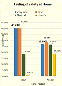
5.1.1. To What Extent Do You Feel Safe at Day/Night Time
During the day, 40.49% of respondents feel very safe and safe at their home, 18.40% responded neutral and 0.16% of respondents feel unsafe. During the night, 26.69% of respondents said they feel very safe at night, compared to 28.22% who said they feel safe, 26.38% who said the safety is neutral, and 18.71% who said they feel unsafe.
Figure 1. Feeling of safety at home.
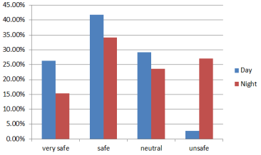
Figure 2. Feeling of safety in neighborhood.
During the day, 26.38% of respondents feel very safe at the neighborhood, 41.72% feel safe while 29.14% responded neutral and 2.76% of respondents feel unsafe. 15.34% of respondents said they feel very safe at night, compared to 34.05% who said they feel safe, 23.62% who said it's neutral, and 26.99% who said they feel.
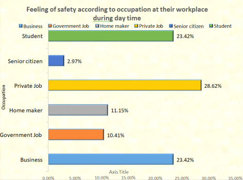
Figure 3. Feeling of safety according to occupation at their workplace during day time.
Assurance of safety According to occupation, we notice that 28.62% of respondents with private jobs feel safe, followed by 23.42% of students and businesspeople and 11.15% and 10.41% of respondents with homemaker and government job responses who feel safe.
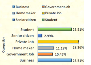
Figure 4. Feeling safe according to workplace during night time.
I can observe that, in terms of workplace safety at night, 28.36% of respondents have private occupations, 23.51% are both students and businesspeople, 11.19% are stay-at-home moms, followed by 10.45% of respondents who work for the government, and 2.99% are senior citizens.
5.1.2. Have You Ever Been a Victim of Crime
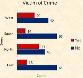
Figure 5. Victim of crime.
In contrast to respondents who answered "No, “I can see from the above map that the majority of respondents in the four zones have ever been the victims of crime?
5.1.3. Have You Ever Registered First Information Report (FIR) for the Crime
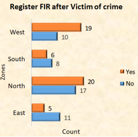
Figure 6. Register FIR after victim of crime.
In contrast to respondents from the south and east, respondents from the west and north zone have registered for the first information report if they have ever been the victims of crime.
5.1.4. If Yes, Did You Get Justice
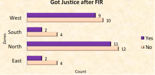
Figure 7. Got justice after FIR.
The graph shows that the majority of respondents who have ever been crime victims and registered for the first information report in the four zones never received justice.
5.1.5. To What Extent Crimes News on Social Media and News Channel Affecting You
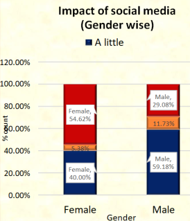
Figure 8. Impact of social media (gender wise).
Here, I observe that 40.0% of females and 59.18% of males are just little impacted by the crime news on social media, compared to 54.62% of females and 29.08% of males who are greatly affected.
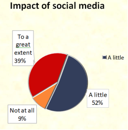
Figure 9. Impact of social media.
Here, 39% of respondents stated they are greatly impacted by the crime news on social media, followed by 52% of respondents who are a little affected, and 9% of respondents claimed they are not at all affected.
5.1.6. How Much CCTV Cameras Are Useful
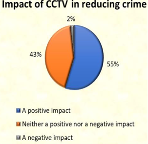
Here, 55% of respondents say that CCTV has a positive impact in reducing crime, 43% say that it has neither a positive or negative impact while 2% say that it has negative impact.
Figure 10. Impact of CCTV in reducing crime.
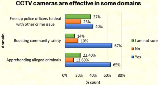
Figure 11. Effectiveness of CCTV cameras in some domain.
The majority of respondents concur that CCTV cameras are effective in boosting community safety, apprehending alleged criminals and free up police officers to deal with other crime issues.
5.1.7. People’s Perception About Police Regarding Their Safety
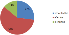
Here, 59% of respondents say that the police are effective, 27% say that the police are very effective and 14% of the respondents say that police are ineffective.
Figure 12. Effectiveness of police in the society.
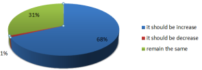
It’s observed that 68% of respondents say that police patrolling should be increase, 31% say that they should stay about the same and 1% say they should be reduced.
Figure 13. What people think about police patrolling.
5.1.8. Is Vadodara a Safe City for Present and Future
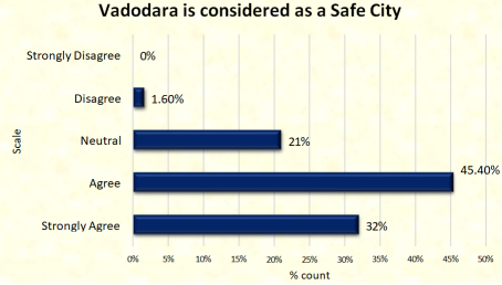
The majority of respondents say that Vadodara is considered as a safe city.
Figure 14. Vadodara is considered as a safe city.
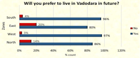
Figure 15. Will you prefer to live in Vadodara in future
The majority of respondents from the four zones agree to live in Vadodara in future.
5.1.9. Have You Ever Taken a Self-defense Course
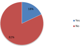
Figure 16. Have you ever taken a self-defense course
Defense training has been taken by 18% of respondents; however 82% have not yet done so.
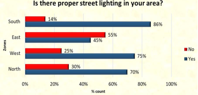
Figure 17. Is there proper street lighting in your area
The majority of respondents agree that the four zones have adequate street lighting, with the south zone leading with 86%, the west zone with 75%, the north zone with 70%, and the east zone with 55%.
5.2. Glimpses of the Secondary Data
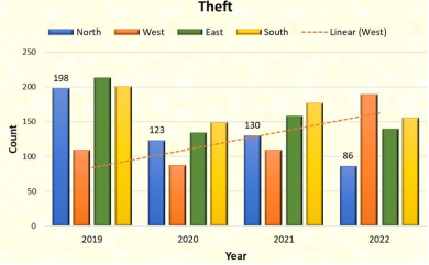
Figure 18. Theft cases zone wise in different years.
Theft crime was the highest recorded in the North and East zone of the city and least recorded in West Zone. In the year 2019 there was the highest number registered of theft crime followed by the year 2022, and least numbers are in year 2020.
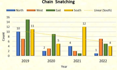
Figure 19. Chain snatching cases zone wise in different years.
The cases of chain snatching were recorded highest in the year 2019 and 2020 in the East zone. In the year 2021, there was sudden increase in the numbers in south zone. In 2022 there is almost similar numbers of the cases of chain snatching in each zone.
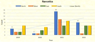
The cases of Narcotics were very less in the year 2019 and 2020 but there was sudden rise in the year 2021 and again it decreased in 2022 year. It happened most in North zone followed by the South zone of the city.
Figure 20. Narcotics cases zone wise in different years.
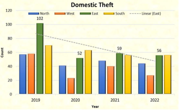
Figure 21. Domestic theft cases zone wise in different years.
The cases domestic theft or burglary was the highest in the East Zone in the year 2019, otherwise the number of cases were almost same in the remaining zones of the mentioned years.
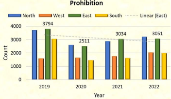
Figure 22. Prohibition cases zone wise in different years.
The highest number of cases recorded in the city of this crime. The number of cases in all zones was higher in the year 2019 except the West zone, in the year 2020 there was decline in number of cases due to COVID-19, in the year 2021 and 2022 there were almost same number of cases in all Zones.
6. Statistical Analysis
6.1. Shapiro-Wilk’s Test for Normality
6.1.1. Testing Normality for Age Data
H0: Age data is normally distributed
H1: Age data is not normally distributed
shapiro.test (data$Age)
Shapiro-Wilk normality test
data: data$Age
W = 0.89889, p-value = 2.79e-15
Here, p-value < 0.05. So, reject the null hypothesis at 5% level of significance. Hence, Age data is NOT normally distributed.
6.1.2. Testing Normality for Number of Family Members’ Data
H0: Number of family member data is normally distributed
H1: Number of family member data is not normally distributed
shapiro.test (data$members)
Shapiro-Wilk normality test
data: data$members
W = 0.49912, p-value < 2.2e-16
Here, p-value < 0.05. So, reject the null hypothesis at 5% level of significance. Hence, number of family members’ data is NOT normally distributed.
6.2. Chi-Square Test of Independence
The Chi-square test of independence (also known as the Pearson Chi-square test, or simply the Chi-square) is used to test for a relationship between two categorical variables. If two variables are independent in the population; samples will vary due to random sampling variation. This test also provides detailed information on exactly which categories account for any differences found.
6.2.1. Assumptions
1) All the variables should be categorical.
2) The study groups should be independent.
3) The groups of the categorical variable must be mutually exclusive.
4) There must be at least 5 expected frequencies in each group of the categorical variable otherwise we need to apply Yates’ correction for continuity (for 2 x 2 contingency table).
6.2.2. Hypothesis
H0: There is no relationship between the two categorical variables i.e., they are independent
H1: There is a relationship between the two categorical variables i.e., they are dependent
Where;
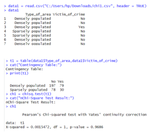
6.2.3. To Check the Association Between Types of Area People Live and Ever Become a Victim of Crime
H0: There is no association between type of area and having been a victim of crime
H1: There is association between type of area and having been a victim of crime
Figure 23. To check association between type of area and having been a victim of crime.
Here, p-value (0.9686) > α (0.05). So, do not reject the null hypothesis at 5% level of significance. Hence, I can conclude that there is no significant association between type of area and ever been a victim of crime.
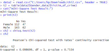
6.2.4. To Check the Association Between Gender and Ever Become a Victim of Crime
H0: There is no association between genders and have been a victim of crime
H1: There is association between genders and have been a victim of crime
Figure 24. To check association between gender and have been a victim of crime.
Here, p-value (0.7534) > α (0.05). So, do not reject the null hypothesis at 5% level of significance. Hence, I can conclude that there is no significant association between gender and ever been a victim of crime.
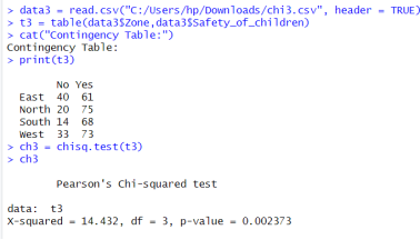
6.2.5. To Check the Association Between Zone and Perception on Safety of Children
Figure 25. To check association between zone and safety of children.
H0: There is no association between zone and safety of children
H1: There is association between zone and safety of children
Here, p-value (0.002) < α (0.05). So, reject the null hypothesis at 5% level of significance. Hence, I can conclude that there is significant association between zone and people perception about safety of children.
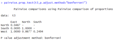
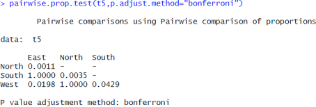
i) Now, I will see pairwise difference in each group by using pairwise proportion test:
Figure 26. Pairwise comparisons using pairwise comparison of proportions test.
Here, p-value for North verses East zone is less than 0.05 i.e., 0.04, so I can say that there are significantly more people in east zone who are more insecure regarding children safety than north zone. Same as with South verses East zone.
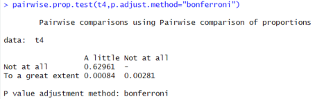
6.2.6. To Check the Association Between Gender and Social Media or News Channel Affects Them
Figure 27. To check association between gender and social media affect.
Ho: There is no association between gender and social media affect
H1: There is association between gender and social media affect
Here, p-value (4.122e-05) < α (0.05). So, reject the null hypothesis at 5% level of significance. Hence, I can conclude that there is significant association between gender and how people have been affected from social media news.
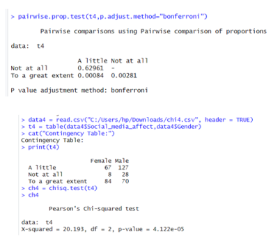
i)Now, I will see pairwise difference in each group by using pairwise proportion test:
Figure 28. Checking which gender is affected much.
The p-value for to a great extent verses a little is less than 0.05 i.e., 0.0008, so I can say that there are significantly more females that are affected much with social media news than males.
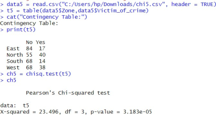
6.2.7. To Check Association Between Zones and Have Been a Victim of Crime
Figure 29. To check association between zones and have been a victim of crime.
Ho: There is no association between zones and have been a victim of crime
H1: There is association between zones and have been a victim of crime
Conclusion: Here, p-value (3.183e-05) < α (0.05). So, reject the null hypothesis at 5% level of significance. Hence, I can conclude that there is significant association between zones and have been victim of crime.
i) Now, I will see pairwise difference in each group by using pairwise proportion test:
Figure 30. Checking how many people have been victim of crime zone wise.
The p-value for north zone verses east zone is less than 0.05 i.e., 0.0011, so I can say that there are significantly more people in north zone have been victim of crime than in east zone.
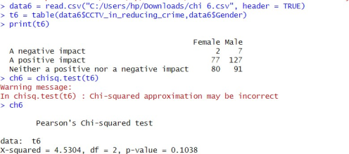
6.2.8. To Check the Association Between Genders and People’s Perception on Impact of CCTV in Reducing Crime
Ho: There is no association between gender and impact of CCTV
H1: There is association between gender and impact of CCTV
Figure 31. Checking association between gender and impact of CCTV.
Conclusion: Here, p-value (0.1038) > α (0.05). So, do not reject the null hypothesis at 5% level of significance. Hence, I can conclude that there is no significant association between gender and their perception on CCTV regarding reducing in crime.
6.3. Rank Analysis
The question that we have used for Rank analysis is given as follows: In your opinion, rank the following crime in order, with one being the most feared to eight being the least feared? [Burglary, Theft, Narcotics, Alcoholic offence, Chain Snatching, Damaged domestic property, Sexual offence, damaged public property].
For the analysis of this ranked data, firstly I have used;
6.3.1. Friedman Test
The Friedman test is a non-parametric statistical test similar to the parametric repeated measure ANOVA; it is used to detect differences in treatments across multiple test attempts.
Test Formula:
Where,
k = the number of groups (treatments)
n = the number of subjects
𝑅𝑗 = the sum of the ranks for the 𝑗𝑡ℎ group
Hypothesis:
Ho: There is no significant difference between respondent ranks.
H1: There is a significant difference between respondent ranks.
Table 2. Friedman Test Statistics for Ranking Differences among Related Groups.
Friedman Test Statistic |
N | 384 |
Chi-Square | 181.291 |
Df | 7 |
Asymp. Sig. | <.001 |
Here, Asymp. Sig. < 0.05, so, reject null hypothesis. I conclude that there is a significant difference between respondent’s ranks.
Now, to find the level of agreement among the individuals who ranked the factors, I have used the Kendall’s coefficient of concordance.
6.3.2. Kendall’s W
Kendall’s W statistic (sometimes called the Coefficient of Concordance) is used to assess agreement between different raters, and in particular inter-rater reliability. It is ranges from 0 to 1; Zero is no agreement at all between raters, while 1 is perfect agreement.
Test Calculation: Assume there are m raters rating k subjects in rank order from 1 to k.
𝑟𝑖𝑗 = the rating rater j gives to subject i.
There are two ways of computing Kendall’s W statistic based on 𝑆 or 𝑆’ but they lead to same result,
Thus,
Where 𝑇 = ⅀(𝑡- 𝑡𝑙) a correction factor is for tied ranks, in which 𝑡𝑙 is the number of tied ranks in each of k groups of ties. The sum is computed over all groups of ties found in all m variables of the data table. When there are no tied values.
If the W Statistic is 0, that means everyone ranked the list differently (or randomly).
If the W Statistic is 1, then everyone ranked the list in exactly the same order.
1) Hypothesis:
H0: there is no agreement among the raters.
H1: there is some agreement among the raters.
Where for a given, is the tabled value obtained from the chi- square table, with k-1 degree of freedom.
2) Analysis
Hypothesis:
H0: There is no agreement among the raters.
H1: There is an agreement among the raters.
Table 3. Test Statistics for Kendall’s Coefficient of Concordance (W) Among Respondents.
Test Statistics |
N | 384 |
Kendall's Wa | 0.067 |
Chi-Square | 181.291 |
df | 7 |
Asymp. Sig. | <.001 |
Here, Asymp. Sig. < 0.05, so, reject null hypothesis. I conclude that there is an agreement among the raters.
Now, to identify factors contribution, I have calculated mean rank of all the factors in SPSS software.
Here, I do a ranking as form of the lowest mean rank has highest rank and the highest mean rank has lowest rank.
6.3.3. Ranks
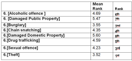
Table 4. Mean Ranks and Ranking of Street Crime Factors Based on Friedman Test Results.
| Mean Rank | Ranking of factors on the basis of means ranks |
[Damaged Domestic Property] | 5.11 | 8th |
[Damaged Public Property] | 5.10 | 7th |
[Burglary] | 3.84 | 2nd |
[Drug trafficking] | 5.01 | 6th |
[Alcoholic offence] | 4.89 | 5th |
[Sexual offence] | 4.47 | 4th |
[Chain snatching] | 4.12 | 3rd |
[Theft] | 3.45 | 1st |
Since, among the other crimes theft has the lowest mean rank i.e. 3.45, it means that respondents are more worried about theft crime and for Damaged Domestic Property respondents are less worried.
Now, I identify zone wise which crime has highest mean rank and which has lowest mean rank.
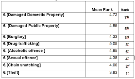
1) Ranking for North Zone
Figure 32. Ranking of Street Crime Types Based on Mean Ranks Using Friedman Test.
Since, for North zone among the other crimes theft has the lowest mean rank i.e. 3.52, it means that respondents are more worried about theft crime and for Damaged Domestic Property, respondents are less worried.
2) Ranking for South Zone
Figure 33. Ranking of Street Crime Types Based on Mean Ranks Using Friedman Test.
Since, for South zone among the other crimes theft has the lowest mean rank i.e.: 2.94, it means that respondents are more worried about theft crime and for Damaged Domestic Property, respondents are less worried.
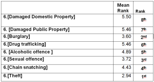
3) Ranking for East Zone
Figure 34. Ranking of Street Crime Types Based on Mean Ranks Using Friedman Test.
Since, for East zone among the other crimes theft has the lowest mean rank i.e. 3.42, it means that respondents are more worried about theft crime and for Sexual offence crime, respondents are less worried.
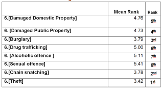
4) Ranking for West Zone
Figure 35. Ranking of Street Crime Types Based on Mean Ranks Using Friedman Test.
Since, for West zone among the other crime theft has the lowest mean rank i.e. 3.83, it means that respondents are more worried about theft crime and for Drug Trafficking, respondents are less worried.
6.4. Multiple Response Analysis
Multiple response analysis is a frequency analysis for data which include more than one response per participant.
To apply this test in SPSS software, we have to follow these following steps:
1) From the menu,
Select Analyze > Multiple Response > Define variable set...
2) Drag and drop required variable sources (this is the descriptive label for the multiple response set $ new variable name) from the variable list into ‘variable in set’ column. The icon next to the "variable" in the variable list identifies it as a multiple dichotomy set. (For a multiple dichotomy set, each "category" is, in fact, a separate variable, and the category labels are the variable labels (or variable names for variables without defined variable labels). In this example, the counts that will be displayed represent the number of cases with a Yes response for each variable in the set.)
3) Then again select: Analyze > Multiple Response > Frequencies...
4) Drag and drop $ new_variable_name into ‘variable in set’ column and then click OK to create the tab
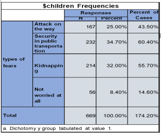
6.4.1. What Are the Parents Fear Regarding Their Kid's Safety
1) Attack on the way
2) Security in public transportation
3) Kidnapping on the way to school
4) Not worried at all
Figure 36. Frequency Distribution of Types of Fears Related to Children’s Safety.
I observe from this analysis that 34.7% Parents has fear about their child Security in public transport, 32% Parents has fear of their child being kidnap, and 25% Parents are worried about their child being attack on the way to school while 8.3% Parents are not worried at all.
6.4.2. Why the Crimes Against Women Are increasing
1) No fear of the law
2) Unsafe and inadequate transport services
3) Lack of police patrolling on the streets
4) Women dressing in skimpy clothes
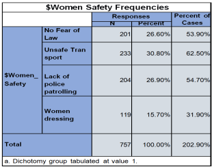
Figure 37. Frequency Distribution of Types of Fears Related to women’s Safety.
I observe from this analysis that; 30.8% respondents feel that due to unsafe transportation crime against women are increasing, 26.6% and 26.9% respondents fell No fear of law and Lack of police patrolling could be the reason of increasing crime against women, while 15.7% respondents feel women dressing is the reason of crime against women are increasing.
6.4.3. What Are the Main Causes of Being Afraid of Burglary or Theft
1) Due to some past experience
2) News coverage of Burglary and theft
3) Due to some other people’s experience
4) Due to inefficient security
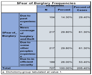
Figure 38. Frequency Distribution of Reasons Behind Fear of Burglary Among Respondents.
I observe from this analysis that; 29.8% respondents fell that the reason of being afraid of burglary and theft are news coverage of the crime and due to some others experience, 26% has fear due to insufficient security, while 14.3% has past experience of burglary or theft that’s why they afraid of this crime.
6.4.4. According to You, How Can You Take the Charge of Your Safety
1) To be aware of your surroundings.
2) To pay attention to the people around you.
3) To react quickly to danger.
4) To flee away from that place.
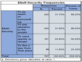
Figure 39. Factors Contributing to Fear of Burglary Among Respondents.
I observe from this analysis that; 31.8% and 31.7% respondents think that to pay attention to the people and too aware of surrounding is the way to take your own safety charge, 24.9% thinks that to react quickly to the danger and 11.6% think that to flee away from that place where you fill unsafe.
6.4.5. What Do You Expect from the Government for Your Safety and Protection
1) Install a security system.
2) Improve lighting on your street.
3) Control of juvenile crime.
4) Dealing with homeless population.
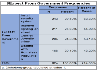
Figure 40. Distribution of Respondents by Reasons for Fear of Burglary.
I observe from this analysis that; 29.5% respondent says that government should install security system, 25.6% and 24.8% says that improve lighting on street and control juvenile crime, while 20.1% says that government should dealing with homeless population for safety and protection of the public.
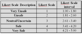
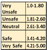
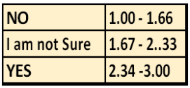
6.5. Likert Scale Analysis
A Likert scale is a rating scale that assesses opinions, attitudes or behaviors quantitatively. It is a 5 or 7-point ordinal scale used by respondents to rate the degree to which they agree or disagree with a statement.
Steps in SPSS
Analyze > Descriptive stats. >Frequencies > (select mean, std) > OK
Qualitative Interpretation of 5-Point Likert Scale Measurements.
Figure 41. Interpretation of Safety Perceptions Using a 5-Point Likert Scale.
6.5.1. To What Extent Do You Feel Safe at Day Time
Very Safe Safe Neutral Unsafe Very Unsafe
1) At home
2) In your neighborhood
3) In your community
4) At your workplace
6.5.2. To What Extent Do You Feel Safe at Night Time
Very Safe Safe Neutral Unsafe Very Unsafe
1) At home
2) In your neighborhood
3) In your community
4) At your workplace
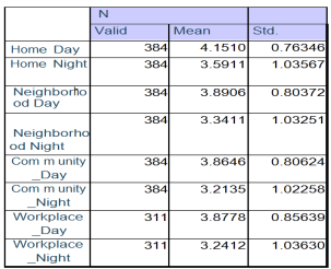
Figure 42. Descriptive Statistics of Perceived Safety in Home, Neighborhood, Community, and Workplace.
Interpretation;
Figure 43. Safety Perception Scale with Interpretation Ranges.
On the basis of above Interpretation scale I conclude that respondents feel safe at home during both Day and night time, respondents feel safe in neighborhood during day time while they feel neutral in night time, respondents feel safe in community during day time while they feel neutral in night time, respondents feel safe at workplace during day time while they feel neutral in night time.
6.5.3. Are the Installed CCTV Cameras Effective in
Yes No I am not sure
1) Apprehending alleged criminals
2) Boosting community safety
3) Free up police to deal with other crime issues
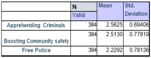
Figure 44. Descriptive statistics of effectiveness of CCTV cameras.
Figure 45. Effectiveness of CCTV Perception Scale with Interpretation Ranges.
On the basis of above interpretation scale, I conclude that Respondents feel that installation of CCTV will helps in apprehending alleged criminals and boosting community safety and they are not sure about the Free up police to deal with Other crime issues.
Multinomial Logistic Regression Model
The MLR tried to find the best fitted model to describe the relationship between the polytomous dependent variable with more than the two categories and one independent variable set.
The logit distribution constrains the estimated probabilities that between 0.0 and 1.0 the logit function can be expressed as:
logit(p)=b0+b1X1+b2X2+….+bkXk
Where,
P: the probability of presence of an outcome of interest.
XK: the vector of K independent variables.
b0: the regression coefficient on the constant term (intercept).
bk: the vector of regression coefficient on the independent variable XK.
The odd ratio is the probability of the event divided by the probability of the non-event and is defined as follows,
Odd ratios
When p = 0 then add (p) = 0, when p = 0.5 then add (p) = 1.0 and when p = 1.0 then add (p) = ∞.
The logit transformation is defined at the logged adds,
Logit (p)
The transformation from adds to log of odds is the log transformation and this is a monotonic transformation. That is, the greater the odds, the greater the log of odds and vice-versa.
Logit (p) can be transformed toby the following formula,
6.6. Multinomial Logistic Regression Analysis
It is a straightforward generalization of binary logistic regression designed to handle situations where the dependent variable has more than two categories. This method relies on maximum likelihood estimation to determine the probability that an observation falls into a particular category.
The logit function can be defined as -:
In this demonstration, I examined predictors of respondent’s prediction of the people’s concern because of continuous hike in fuel prices using Multinomial Logistic Regression.
The dataset contains 384 observations. The reference category or the dependent variable is how much people are worried to become a victim of crime which is going to be measured in three levels - Very worried, little worried and not worried.
The predictors or independent variable included:
1) Have you ever been a victim of crime
2) Social media or news channel affecting you
3) Proper street lightning
4) Zone
5) Gender
6) Occupation
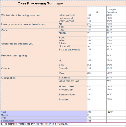
6.6.1. Case Processing Summary
This is a summary with various descriptions of our data.
N provides the number of observations fitting the description in the first column.
The marginal percentage lists the proportion of valid observations found in each of the outcome variable’s groups. This can be calculated by dividing the N for each group by the N for “Valid”.
A subpopulation of the data consists of one combination of the predictor variables specified for the model.
Figure 46. Case processing summary.
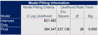
6.6.2. Model Fitting Information
It represents discrepancies between observed and model-implied data.
It describes the relationship between a response variable and one or more predictor variables.
Ho: There is no significance difference between null model (model with intercept only) and final model (model with all the variables).
H1: There is a significance difference between null model (model with intercept only) and final model (model with all the variables).
Figure 47. Model fitting information.
The model fitness assessed using the chi-square statistic. The Chi-Square value is 237.136 and the p-value less than 0.05. This proves that there is a significant relationship between the dependent and independent variables in the final model.
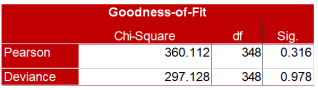
6.6.3. Goodness-of-Fit Test
The Goodness-of-Fit table provides two measures that can be used to assess how well the model fits the data, as shown below:
Ho: The model fits adequately
H1: The model does not fit adequately
Figure 48. Goodness-of-fit test.
The first row, labeled "Pearson", presents the Pearson chi-square statistic. From the table above that the p-value is .316 (i.e. =.316 > 0.05. So, do not reject Ho). Based on this measure, the model fits the data well.
The other row of the table (i.e., the "Deviance" row) presents the Deviance chi-square statistic and its p - value is 0.978.
It proves that the model is fit.
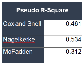
6.6.4. Pseudo R- Square
A pseudo-R-squared only has meaning when compared to another pseudo-R-squared of the same type, on the same data, predicting the same outcome. In this situation, the higher pseudo-R-squared indicates which model better predicts the outcome.
Figure 49. Pseudo R-Square.
The model accounts for 31% to 53% of the variance and represents relatively decent sized effects.
According to McFadden’s test we can say that full model containing our predictors represents a 31% improvement in fit relative to the null model.
6.6.5. Likelihood Ratio Test
A likelihood ratio test compares the goodness of fit of two nested regression models.
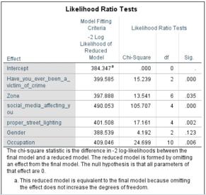
Figure 50. Likelihood Ratio Test.
The likelihood ratio proves that the past experience of victim of crime, social media, proper street lighting, zone and occupation are more significant than other variables which proves that these predictors contribute significantly to the final model.
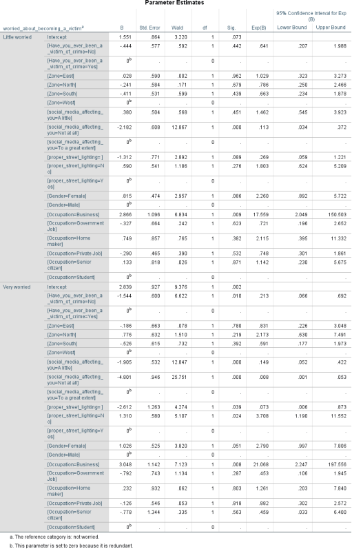
Figure 51. Parameter estimates.
Parameter Estimates
B is the estimated coefficient, with standard error, S. E. c. The ratio of B to S. E., squared, equals the Wald statistic.
If the Wald statistic is significant (i.e., less than 0.05) then the parameter is useful to the model. d. “Exp (B),” or the odds ratio, is the predicted change in odds for a unit increase in the predictor.
The “exp” refers to the exponential value of B. When Exp (B) is less than 1, increasing values of the variable correspond to decreasing odds of the event's occurrence. When Exp (B) is greater than 1, increasing values of the variable correspond to increasing odds of the event's occurrence. If you subtract 1 from the odds ratio and multiply by 100, you get the percent change in odds of the dependent variable having a value of 1.
The probability of people who have no much effect of social media are little worried with respect to not worried is 0.113 times higher than the other.
The probability of people whose occupation is business are little worried w.r.t. to not worried is 17.559 times higher than the other occupation.
The probability of people who are not victim of crime are little worried w.r.t. not worried is 0.149 times higher than the other groups.
The probability of people who have no much effect of social media are very worried w.r.t. to not worried is 0.008 times higher than the other.
The probability of people who have no much effect of social media are very worried w.r.t. to not worried is 0.113 times higher than the other.
The probability of people who respond their area has no proper street lighting are very worried w.r.t. to not worried is 0.081 higher than the other.
7. Conclusions
According to the survey, 40.49% of respondents said they feel very safe and safe at home during the day, 18.40% gave a neutral response and 0.16% said they feel unsafe. Again, 26.69% of respondents reported feeling very safe at home at night, compared to 28.22% who reported feeling safe, 26.38% who reported the safety as neutral, and 18.71% who reported feeling unsafe.
According to the study, 26.38% of respondents said they feel very safe in their neighborhood during the day, followed by 41.72% who said they feel safe, 29.14% who felt neutral, and 2.76% who said they feel unsafe. 15.34% of respondents said they feel very safe in the neighborhood at night, compared to 34.05% who said they feel safe, 23.62% who said it's neutral, and 26.99% who said they feel safe.
26.07% of respondents said they feel very safe in the community throughout the day, 41.41% said they feel safe, 29.45% said they felt neutral, and 3.07% said they feel unsafe. 10.74% of participants reported feeling very safe at night, compared to 24.23% who reported feeling safe, 29.14% who reported it as neutral, and 1.23% who reported feeling unsafe.
During the day, 26.38% of respondents said they feel very safe at the work, 26.07% feel safe while 28.53% responded neutral and 1.53% of respondents feel unsafe. 9.82% of respondents said they feel very safe at night, compared to 27.91% who said they feel safe, 22.70% who said it's neutral and 21.47% who said they feel unsafe.
Assurance of safety According to occupation, we notice that 28.62% of respondents with private jobs feel safe, followed by 23.42% of students and businesspeople, 11.15% of homemakers, and 10.41% of those working for the government responded they feel safe.
I can observe that, in terms of workplace safety at night, 28.36% of respondents who feel safe are those with private occupations, 23.51% are both students and businesspeople, 11.19% are stay-at-home moms, followed by 10.45% of respondents who work for the government, and 2.99% are senior citizens.
According to being a victim of crime, in contrast to respondents who answered "No," I can see from the above map that the majority of respondents in the four zones have ever been the victims of crime.
I discovered that respondents from the west and north zones, in contrast to those from the south and east, have registered for the first information report if they have ever been the victims of crime.
From the survey, we discovered that the majority of respondents who had ever been crime victims and registered for the initial information report in the four zones never obtained justice.
Here, 39% of respondents stated they are greatly impacted by the crime news on social media, followed by 52% of respondents who are a little affected, and 9% of respondents claimed they are not at all affected.
About the impact of CCTV in reducing crime, 55% of respondents say that CCTV has a positive impact in reducing crime, 43% say that it has neither a positive or negative impact while 2% say that it has negative impact.
The majority of respondents concur that CCTV cameras are effective in boosting community safety, apprehending alleged criminals and free up police officers to deal with other crime issues.
Regarding the effectiveness of police in the society, 59% of respondents responded that the police are effective, 27% said that the police are very effective and 14% of the respondents said that police are ineffective.
According to respondents' perceptions of police patrolling, 68% believe it should be increased, 31% believe it should remain roughly the same and 1% believe it should be decreased.
Concerning the availability of self-defense training, 82% of respondents have not yet participated in self-defense training, compared to 18% of respondents who have.
The majority of respondents believe that each of the four zones has sufficient street lighting, with the south zone leading the way with 86%, followed by the west zone with 75%, the north zone with 70%, and the east zone with 55%.
Vadodara is a safe city, according to most survey participants. From the four zones, the most majority of respondents concur that they will move to Vadodara in the future.
The North and East zones of the city had the most and the West zone had the least theft crimes reported. The most theft crimes were reported in 2019, then in 2022, and in 2020.
In the East zone, the most instances of chain snatching were reported in the years 2019 and 2020. The numbers in the south zone suddenly increased in the year 2021. In each zone, the number of chain snatching incidents in 2022 is nearly equal.
The use of drugs was extremely low in 2019 and 2020, and then it suddenly increased in 2021 before falling off again in 2022. The North zone of the city experienced the highest rate of occurrence, followed by the South zone.
The highest number of prohibition cases ever reported in the city occurred in 2019, when cases in all zones except the West zone were higher. Following a decline in cases in 2020 as a result of COVID-19, cases in all zones were nearly equal in number in 2021 and 2022.
In 2019, the East Zone had the highest number of cases of domestic theft or burglary; otherwise, the number of cases in the other zones during those years was essentially the same.