Applications of Adaptive Filtering Techniques for Noise Cancellation Systems to the Ultrasonic Non-Destructive Evaluation (NDE)

Birtukan Yenealem; Mamaru Genetu; Elias Mamushet

doi:doi:10.11648/j.jeee.20251304.13

Research Article |

| Peer-Reviewed

Applications of Adaptive Filtering Techniques for Noise Cancellation Systems to the Ultrasonic Non-Destructive Evaluation (NDE)

Birtukan Yenealem

, Mamaru Genetu^*

, Elias Mamushet

Published in Journal of Electrical and Electronic Engineering (Volume 13, Issue 4)

Received: 28 May 2025 Accepted: 16 June 2025 Published: 28 July 2025

Views: Downloads:

Download PDF

Share This Article

Twitter
Linked In
Facebook

Abstract

The performance of ultrasonic non-destructive evaluation (NDE) systems is frequently limited by backscattering and electronic noise, which reduce sensitivity and resolution, particularly in industrial environments. At the Metals Industry Development Institute in Ethiopia, the ultrasonic NDT flaw detector (model UFD-01/T) has been employed to defects internal material defects. However, accurately pinpointing crack related frequencies remains difficult due to substantial environmental noise interference. To address this challenge, a post-processing noise cancellation system was developed utilizing advanced adaptive filtering techniques. This study presents mathematical models for noise reduction and evaluates the effectiveness of several adaptive filter algorithms, including Fast Fourier Transform (FFT), Finite Impulse Response (FIR), Infinite Impulse Response (IIR), and Least Mean Square (LMS) methods. These algorithms were implemented and simulated within the MATLAB environment to assess their ability to isolate defect signals from noise. Simulation results demonstrate that the proposed adaptive filtering methods, particularly the LMS algorithm, effectively attenuate high-frequency noise originating from echoes and environmental interferences. Consequently, the noise floor in the processed ultrasonic signals was reduced to below 35 dBm, significantly enhancing the capability to localize material defects. These findings support the integration of adaptive filtering techniques in ultrasonic NDE systems to improve defect detection precision in noisy industrial environments, thereby enhancing inspection reliability, reducing false positives, and contributing to the overall safety and efficiency of industrial operations.

Published in	Journal of Electrical and Electronic Engineering (Volume 13, Issue 4)
DOI	10.11648/j.jeee.20251304.13
Page(s)	168-183
Creative Commons	This is an Open Access article, distributed under the terms of the Creative Commons Attribution 4.0 International License (http://creativecommons.org/licenses/by/4.0/), which permits unrestricted use, distribution and reproduction in any medium or format, provided the original work is properly cited.
Copyright	Copyright © The Author(s), 2025. Published by Science Publishing Group

Keywords

NDE, Noise Cancellation, Adaptive Filtering, FFT, Simulation

1. Introduction

Ultrasonic non-destructive evaluation (NDE) is widely used for detecting internal defects in materials, particularly in the metals industry. However, the effectiveness of ultrasonic NDE systems often compromised by various environmental and electronic noise sources, such as welding and acoustic noise, which can significantly corrupt the acquired ultrasonic signals

[1-3]

. Numerous studies have explored noise reduction techniques across diverse applications, including speech processing and machinery, employing methods such as the least squares algorithm to minimize noise impact

[4-7]

. Recent advancements have also introduced FPGA-based finite impulse response (FIR) filter architectures

[8-10]

and register transfer level (RTL) algorithm implementations

[11-14]

for enhanced ultrasonic signal processing. Hybrid approaches that combine multiple signal processing techniques recommended for further improvement.

The surface layer of materials, due to its unique exposure to environmental interactions, mechanical treatments, and stress concentrations, often exhibits properties distinct from the bulk material. These surface characteristics are critical in product design and reliability, making accurate defect detection essential

[15-17]

Despite the progress in mathematical modeling and hardware implementation for noise reduction, previous works have not fully addressed the potential of matched filtering in ultrasonic NDE, particularly for coarse-grained materials. Matched filtering, when properly designed and optimized to approximate defect echoes, offers a powerful and efficient means to enhance defect detection and imaging

[18, 19]

This paper presents the design and simulation of adaptive filtering techniques, including matched filtering, for noise cancellation in ultrasonic NDE applications. The proposed approach incorporates Fast Fourier Transform (FFT), FIR, infinite impulse response (IIR), and least mean square (LMS) algorithms, all implemented and tested in a MATLAB environment.

2. Mathematical Model

This section presents the mathematical framework for noise cancellation in ultrasonic signals using digital adaptive filtering techniques. The goal is to design filters that can effectively separate the desired ultrasonic echoes from unwanted noise, including environmental and electronic interference.

2.1. Signal Model

The signal model provides a foundational framework for ultrasonic signal recovery, where the observed signal x(n)x(n) combines the desired defect echoes s(n)s(n) and additive noise v(n)v(n). This model assumes noise arises from environmental or electronic sources, which can obscure defect detection in non-destructive testing (NDT) applications. Noise characteristics: v(n)v(n) may exhibit Gaussian or non-Gaussian distributions, influencing the choice of recovery techniques. For example, higher-order spectral analysis effectively suppresses Gaussian noise, while matched filtering enhances signal-to-noise ratios in colored-noise environments. Sparsity-based approaches: Compressive sensing methods exploit the inherent sparsity of defect signals in a specific domain.

Let the acquired ultrasonic signal be modeled as:

𝑥(𝑛)=𝑠(𝑛)+𝑣(𝑛)x(n)=s(n)+v(n)

Where,(𝑛)x(n):- observed (noisy) signal; (𝑛)s(n):- desired ultrasonic signal (echoes from defects); (𝑛)v(n):- unwanted noise (environmental/electronic).

The objective is to recover (𝑛)s(n) from 𝑥(𝑛)x(n) by minimizing the noise 𝑣(𝑛)v(n).

2.2. Adaptive Filtering Framework

An adaptive filter dynamically adjusts its parameters to minimize the error between a desired reference signal (𝑛)d(n) and the filter output 𝑦(𝑛)y(n). The error signal defined as:

𝑒(𝑛)=𝑑(𝑛)−𝑦(𝑛)e(n)=d(n)−y(n)

The filter output is given by:

𝑦(𝑛)=𝑤𝑇(𝑛)𝑥(𝑛)y(n)=wT(n)x(n)

Where,

1) 𝑤(𝑛)=[𝑤0(𝑛), 𝑤1(𝑛),...,𝑤𝐿−1(𝑛)]𝑇w(n)=[w0(n), w1(n),..., wL−1(n)] T: adaptive filter coefficients (L-tap)

2) 𝑥(𝑛)=[𝑥(𝑛),𝑥(𝑛−1),...,𝑥(𝑛−𝐿+1)]𝑇x(n)=[x(n), x(n−1),..., x(n−L+1)] T: input signal vector

The filter coefficients updated to minimize the mean square error (MSE):

(𝑛)=[𝑒2(𝑛)]J(n)=E[e2(n)]

2.3. Least Mean Square (LMS) Algorithm

The LMS algorithm is a widely used adaptive filtering method due to its simplicity and robustness. The coefficient update rule is:

𝑤(𝑛+1)=𝑤(𝑛)+𝜇𝑒(𝑛)𝑥(𝑛)w(n+1)=w(n)+μe(n)x(n)

Where,

1) 𝜇μ: step-size parameter (controls convergence and stability)

2) (𝑛)e(n): error signal

The LMS algorithm iteratively adjusts the filter weights to minimize the MSE, enabling real-time noise cancellation in ultrasonic NDE applications.

2.4. Frequency Domain Analysis Using FFT

To analyze and process signals in the frequency domain, the Fast Fourier Transform (FFT) is applied:

[𝑘]=∑𝑛=0𝑁−1[𝑛]𝑒−𝑗2𝜋𝑁𝑘𝑛,𝑘=0,1,...,𝑁−1X[k]=n=0∑N−1x[n]e−jN2πkn,k=0,1,...,N−1

FFT efficiently decomposes the signal into its constituent frequencies, facilitating the identification and suppression of noise components.

2.5. FIR and IIR Filter Models

Finite Impulse Response (FIR) Filter:

(𝑛)=∑𝑖=0𝐿−1ℎ(𝑖)𝑥(𝑛−𝑖)y(n)=i=0∑L−1h(i)x(n−i)

Where, ℎ (𝑖) h (i) are the filter coefficients.

Infinite Impulse Response (IIR) Filter:

𝑦(𝑛)=∑𝑖=0𝑀𝑎(𝑖)𝑥(𝑛−𝑖)−∑𝑗=1𝑁𝑏(𝑗)𝑦(𝑛−𝑗)y(n)=i=0∑Ma(i)x(n−i)−j=1∑Nb(j)y(n−j)

Where, (𝑖)a(i) and 𝑏(𝑗)b(j) are the filter coefficients.

Both FIR and IIR filters can be used as part of the adaptive filtering framework, with FIR filters offering guaranteed stability and IIR filters providing efficient realization of sharp frequency responses.

2.6. Implementation and Practical Considerations

The proposed adaptive noise cancellation system implemented and tested using MATLAB/Simulink with signals acquired from ultrasonic sensors on metallic samples. The algorithms designed to operate in real-time, addressing challenges such as computational cost and the need for rapid convergence.

Simulation and experimental results confirm that the adaptive filtering approach-particularly the LMS algorithm-effectively suppresses high-frequency noise, yielding a filtered signal with a noise floor below 35 dBm and significantly improving defect localization.

This mathematical modeling framework demonstrates how digital adaptive filtering, combined with frequency domain analysis, can be systematically applied to enhance ultrasonic NDE signal quality by removing unwanted noise components.

2.7. The Fast Fourier Transform (FFT) Algorithm

General Definition of FFT

X[k] = ∑_{n=0}^{N-1} x[n]e^{-j\frac{2\pi}{N}kn}, k = 0,1,…N-1(1)

For each k value, this requires:

N complex multiplications

N-1 complex additions

O(N²) computations for direct DFT

FFT Optimization Principles

FFT exploits symmetries of e^{-j\frac{2\pi}{N}kn} by defining W_N = e^{-j\frac{2\pi}{N}}

Complex conjugate symmetry: W_N^{k(N-n)} = W_N^{-kn} = (W_N^{kn})*

Periodicity in n, k: W_N^{kn} = W_N^{k(N+n)} = W_N^{(k+N)n}

Decimation in Time FFT

Building a large DFT from smaller ones (assuming N = 2^m):

Separate x[k] into even and odd-indexed subsequences:

X[k] = ∑{n=0}^{N-1} x[n]W_N^{kn} = ∑{even} x[n]W_N^{kr} + ∑_{odd} x[n]W_N^{kr}(2)

Where even indices are:

n = 2r

n = 2r+1

r = 0, 1, 2,..., N/2-1

This gives:

X[k] = ∑{r=0}^{N/2-1} x[2r]W_N^{k2r} + ∑{r=0}^{N/2-1} x(2r+1)W_N^{(2r+1)k}(3)

Rearranging:

X[k] = ∑{r=0}^{N/2-1} x2r^{kr} + W_N^k ∑{r=0}^{N/2-1} x2r+1^{kr}(4)

Since W_N^2 = e^{-j\frac{2\pi}{N}2} = e^{-j\frac{2\pi}{N/2}} = W_{N/2}(5)

We can rewrite:

X[k] = ∑{r=0}^{N/2-1} x[2r]W{N/2}^{kr} + W_N^k ∑{r=0}^{N/2-1} x[2r+1]W{N/2}^{kr}(6)

X[k] =∑𝑁−1 [𝑛]−j 2𝜋𝑘𝑛,𝑘= 0,1, ….𝑁–1

𝑛=0 𝑁

X[k] = ∑{r=0}^{N/2-1} x[2r]W{N/2}^{kr} + W_N^k ∑{r=0}^{N/2-1} x[2r+1]W{N/2}^{kr}(7)

X[k] =∑𝑁−1 [𝑛]−j 2𝜋𝑘𝑛,𝑘= 0,1, ….𝑁− 1

𝑛=0 𝑁

2.8. Fast Fourier Transform (FFT) and DFT Decomposition

The Discrete Fourier Transform (DFT) of a sequence [𝑛] x[n] of length 𝑁N is defined as:

𝑋[𝑘]=∑𝑛=0𝑁−1𝑥[𝑛]𝑒−𝑗2𝜋𝑁𝑘𝑛,𝑘=0,1,…,𝑁−1(1)X[k]=n=0∑N−1x[n]e−jN2πkn,k=0,1,…,N−1

For each 𝑘k, this requires 𝑁N complex multiplications and 𝑁−1N−1 complex additions, resulting in (𝑁2)O(N2) computations for direct DFT.

The FFT algorithm exploits the symmetry and periodicity properties of the complex exponential to reduce computational complexity. Let 𝑊𝑁=𝑒−𝑗2𝜋𝑁WN=e−jN2π, then:

1) Complex conjugate symmetry

(𝑁−𝑛)=𝑊𝑁−𝑘𝑛=(𝑊𝑁𝑘𝑛)∗WNk(N−n)=WN−kn=(WNkn)*

2) Periodicity: 𝑊𝑁𝑘𝑛=𝑊𝑁(𝑁+𝑛)WNkn=WNk(N+n)

Decimation-in-Time FFT

Assuming 𝑁=2𝑚N=2m, the sequence can be separated into even and odd-indexed components:

𝑋[𝑘]=∑𝑟=0𝑁/2−1𝑥[2𝑟]𝑊𝑁𝑘(2𝑟)+∑𝑟=0𝑁/2−1𝑥[2𝑟+1]𝑊𝑁𝑘(2𝑟+1)(2)X[k]=r=0∑N/2−1x[2r]WNk(2r)+r=0∑N/2−1x[2r+1]WNk(2r+1)(2)=∑𝑟=0𝑁/2−1𝑥[2𝑟]𝑊𝑁/2𝑘𝑟+𝑊𝑁𝑘∑𝑟=0𝑁/2−1𝑥[2𝑟+1]𝑊𝑁/2𝑘𝑟(3)=r=0∑N/2−1x[2r]WN/2kr+WNkr=0∑N/2−1x[2r+1]WN/2kr(8)

where 𝑊𝑁/2=𝑒−𝑗2𝜋𝑁/2WN/2=e−jN/22π.

Let:

[𝑘]=∑𝑟=0𝑁/2−1[2𝑟]𝑊𝑁/2𝑘𝑟Xe[k]=∑r=0N/2−1x[2r]WN/2kr(9)

[𝑘]=∑𝑟=0𝑁/2−1[2𝑟+1]𝑊𝑁/2𝑘𝑟Xo[k]=∑r=0N/2−1x[2r+1]WN/2kr(10)

Thus, the DFT can be expressed as:

[𝑘]=[𝑘]+𝑊𝑁𝑘𝑋𝑜[𝑘](6)X[k]=Xe[k]+WNkXo[k](11)

where 𝑋𝑒[𝑘] Xe[k] is the DFT of the even samples and 𝑋𝑜[𝑘] Xo[k] is the DFT of the odd samples.

2.9. Transfer Function and Time Domain Equations

After obtaining the transfer function in the Z-domain, the time-domain difference equation derived for digital filter implementation.

Example Transfer Function:

(𝑧)=−2.91×10−16+0.5074𝑧−1+0.1985𝑧−21−0.536𝑧−1+0.3055𝑧−2−0.05514𝑧−3(7)H(z)=1−0.536z−1+0.3055z−2−0.05514z−3−2.91×10−16+0.5074z−1+0.1985z−2(12)

Factored Form:

𝐻(𝑧)=(𝑧−0.072)(𝑧−0.069)(𝑧−0.15±0.46𝑖)(𝑧+0.069)𝑧2−0.003𝑧−0.005(8)H(z)=z2−0.003z−0.005(z−0.072)(z−0.069)(z−0.15±0.46i)(z+0.069)(13)

General Second-Order System:

(𝑠)=(𝑠+𝑎)2+𝑐2(9)H(s)=(s+a)2+c2C(14)

(𝑠)=(𝑠+𝑎)2+𝑐2+𝑠+𝑎(𝑠+𝑎)2+𝑐2(10)H(s)=(s+a)2+c2C+(s+a)2+c2s+a(15)

Z-Transform Pair (from Laplace/Z tables):

𝑍{𝑒−𝑎𝑡sin⁡(𝑤𝑑𝑡)}=𝑧𝑒−𝑎𝑡sin⁡(𝑤𝑑𝑡)𝑧2−2𝑧𝑒−𝑎𝑡cos⁡(𝑤𝑑𝑡)+𝑒−2𝑎𝑡(11)Z{e−atsin(wdt)}=z2−2ze−atcos(wdt)+e−2atze−atsin(wdt)(11)𝑍{𝑒−𝑎𝑡cos⁡(𝑤𝑑𝑡)}=𝑧(𝑧−𝑒−𝑎𝑡cos⁡(𝑤𝑑𝑡))𝑧2−2𝑧𝑒−𝑎𝑡cos⁡(𝑤𝑑𝑡)+𝑒−2𝑎𝑡(12)Z{e−atcos(wdt)}=z2−2ze−atcos(wdt)+e−2atz(z−e−atcos(wdt))(16)

Where 𝑤𝑑𝑡=2𝜋𝑓𝑛wdt=2πfn.

Thus, the time-domain function for the filtered signal is:

𝑥[𝑛]=𝑒−𝑎𝑛[sin⁡(2𝜋𝑓𝑛)+cos⁡(2𝜋𝑓𝑛)](13)x[n]=e−an[sin(2πfn)+cos(2πfn)](17)

2.10. Adaptive Filtering and LMS Algorithm

The output of an adaptive filter can be written as:

𝑦(𝑛)=∑𝑖=0𝐿−1𝑤𝑖(𝑛)𝑥(𝑛−𝑖)=𝑤𝑇(𝑛)𝑥(𝑛)(14)y(n)=i=0∑L−1wi(n)x(n−i)=wT(n)x(n)(18)

where:

1) 𝑤(𝑛)=[𝑤0(𝑛),𝑤1(𝑛),...,𝑤𝐿−1(𝑛)]𝑇w(n)=[w0(n), w1(n),..., wL−1(n)] T is the vector of filter coefficients,

2) 𝑥(𝑛)=[𝑥(𝑛),𝑥(𝑛−1),...,𝑥(𝑛−𝐿+1)]𝑇x(n)=[x(n), x(n−1),..., x(n−L+1)] T is the input vector.

The error signal is:

𝑒(𝑛)=𝑑(𝑛)−𝑦(𝑛)(15)e(n)=d(n)−y(n)(19)

The mean square error (MSE) cost function is:

𝐽(𝑛)=𝐸[𝑒2(𝑛)](16)J(n)=E[e2(n)](20)

To minimize (𝑛)J(n), set its gradient to zero:

∂(𝑛)∂𝑤(𝑛)=0(17)∂w(n)∂J(n)=0(21)

The optimal weights are:

𝑤𝑜𝑝𝑡(𝑛)=𝑅−1(𝑛)𝑟(𝑛)(18)wopt(n)=R−1(n)r(n)(22)

where 𝑅R is the autocorrelation matrix and 𝑟r is the cross-correlation vector.

LMS Algorithm Update Rule:

𝑤(𝑛+1)=𝑤(𝑛)+𝜇𝑒(𝑛)𝑥(𝑛)(19)w(n+1)=w(n)+μe(n)x(n)(23)

where 𝜇μ is the step size.

Summary Table of Key Equations:

Equation Description

(1)-(7) FFT/DFT decomposition and recursion

(8)-(14) Transfer function and time-domain transformation

(15)-(20) Adaptive filter output, error, cost, and LMS update

Note:

1) All variables are defined at their first appearance.

2) Each equation is referenced and explained in context.

3) This arrangement ensures clarity and logical progression from frequency domain analysis (FFT), through system modeling (transfer function), to adaptive filtering (LMS).

2.11. Filtering Process and Adaptive Algorithms

In digital signal processing for ultrasonic NDE, the filtering process can utilize either Finite Impulse Response (FIR) or Infinite Impulse Response (IIR) filters. FIR filters are commonly preferred in many applications due to their inherent stability and use of only forward paths. In contrast, IIR filters can achieve sharper frequency responses with fewer coefficients but may be less stable if not properly designed.

Adaptive filters dynamically adjust their coefficients to minimize the error between the filter output and a desired reference signal. Several algorithms are available for adaptive weight control, including the Least Mean Square (LMS), Delayed LMS (DLMS), Recursive Least Squares (RLS), and Normalized LMS (NLMS) algorithms. Among these, the LMS algorithm is widely used because of its simplicity, low computational requirements, and robust performance.

The output of an adaptive filter, (𝑛)y(n), at time 𝑛n can be expressed as:

𝑦(𝑛)=∑𝑖=0𝐿−1𝑤𝑖(𝑛) 𝑥(𝑛−𝑖)=𝑤𝑇(𝑛) 𝑥(𝑛)y(n)=i=0∑L−1wi(n)x(n−i)=wT(n)x(n)

where:

1) 𝑤(𝑛)=[𝑤0(𝑛),𝑤1(𝑛),…,𝑤𝐿−1(𝑛)]𝑇w(n)=[w0(n), w1(n),…, wL−1(n)] T is the vector of time-varying filter coefficients for an 𝐿L-tap filter,

2) 𝑥(𝑛)=[𝑥(𝑛),𝑥(𝑛−1),…,𝑥(𝑛−𝐿+1)]𝑇x(n)=[x(n), x(n−1),…, x(n−L+1)] T is the input signal vector,

3) (⋅)(⋅) T denotes the transpose operation.

The filter coefficients (𝑛)w(n) are updated to minimize the mean square error (MSE) cost function:

(𝑛)=[𝑒2(𝑛)]J(n)=E[e2(n)]

where 𝑒(𝑛)=𝑑(𝑛)−𝑦(𝑛)e(n)=d(n)−y(n) is the error between the desired signal 𝑑(𝑛)d(n) and the filter output 𝑦(𝑛)y(n).

The optimal filter coefficients can be found by setting the gradient of the cost function with respect to 𝑤(𝑛)w(n) to zero:

∂(𝑛)∂𝑤(𝑛)=0∂w(n)∂J(n)=0

which yields:

𝑤opt(𝑛)=𝑅−1(𝑛) 𝑟(𝑛)wopt(n)=R−1(n)r(n)

where 𝑅(𝑛)R(n) is the autocorrelation matrix of the input signal and 𝑟(𝑛)r(n) is the cross-correlation vector between the input and desired signals.

However, computing the matrix inverse for every new data sample is computationally intensive. Therefore, iterative algorithms such as LMS are typically used for real-time adaptive filtering.

Least Mean Square (LMS) Algorithm

The LMS algorithm updates the filter coefficients iteratively using the following rule:

𝑤(𝑛+1)=𝑤(𝑛)+𝜇 𝑒(𝑛) 𝑥(𝑛)w(n+1)=w(n)+μe(n)x(n)

where:

1) 𝜇μ is the step-size parameter, controlling the convergence rate and stability (0<𝜇<12𝑁𝑅0<μ<2NR1, where 𝑁N is the number of filter taps and 𝑅R is the input signal covariance),

2) (𝑛)e(n) is the instantaneous error.

The LMS algorithm is based on the principle of minimizing the mean square error using a stochastic gradient descent approach. Its main advantages include computational efficiency, ease of implementation, and reliable convergence under stationary conditions.

FIR filters, combined with adaptive algorithms such as LMS, provide an effective and stable solution for noise cancellation in ultrasonic NDE applications. The LMS algorithm, in particular, is favored for its simplicity and real-time capability, making it suitable for practical implementations where computational resources are limited.

Where the vector W(n) [W0 (n) W1 (n) …………WL-1 (n)] T denotes the coefficients of the time-varying L-tap adaptive filter, x(n) [x0 (n) x1 (n)……. x(n-L+1) (n)] T denotes the filter Input vector, and [.] J denotes the transpose operation.

The filter coefficients, W(n), are adjusted to minimize the mean square error function of the system, J (n), given by

J (n)=E[(e2)]

E[d(n)]-WT (n)E[x(n) d(n)]- E [d (n) XT(n)]w(n)+wT(n)E[x(n)xT(n)]w(n)

=E[d2(n)]-2WT(n)rdx(n) + WT(n)rxx(n) w(n)

Where auto correlation matrix is defined by Rxx (n) =E[x (n) d (n)]

To do so, the partial derivative of J (n) with respect to the filter coefficients, W(n) is set to zero.

\frac{\partial J (n)}{\partial w (n)} = 0

(24)

The solution of equation (3) can be written as

Wopt(n)=R -1(n)r (n)(25)

Download: Download full-size image

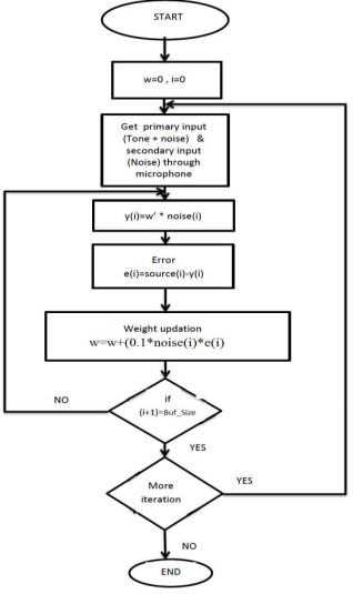
Figure 1. Flow chart of adaptive noise canceller.

The computation cost of equation 4 is enormous due to the matrix inversion calculation for every new data sample. Therefore, an iterative strategy commonly used to update the filter coefficients, W (n).

Figure 1 shows the fundamental algorithm of noise cancellation, Least Mean Square (LMS) algorithm enhanced with adaptive filter. The simulation of the noise cancellation using LMS adaptive filter algorithm is developed. The noise corrupted speech signal and the engine noise signal used as inputs for LMS adaptive filter algorithm. The filtered signal is compare to the original noise-free speech signal in order to highlight the level of attenuation of the noise signal. The result shows that the noise signal successfully canceled by the developed adaptive filter. The difference of the noise-free speech signal and filtered signal are calculated and the outcome implies that the filtered signal is approaching the noise-free speech signal upon the adaptive filtering. The frequency range of the successfully canceled noise by the LMS adaptive filter algorithm is determined by performing Fast Fourier Transform (FFT) on the signals. The LMS adaptive filter algorithm shows significant noise cancellation at lower frequency range.

2.12 LMS Algorithm

The LMS algorithm based on the principle of Minimum Mean square error and the steepest descent algorithms. The main advantages of the LMS algorithm is its Computational simplicity, ease of implementation, unbiased convergence, and the existence of a proof in stationary environment. The following mathematical model describes the LMS algorithm.

y(n) = wT(n).x(n) e(n) = d(n) - y(n) w(n+1) = w(n)+µe(n)x(n)

Where:- y (n) is the filter output, wT (n) is the filter weights in transposed form, x(n) is the filter inputs, d(n)is the desired filter output, e(n) is the error signal which is used for training the filter weights and µ is the step size factor which is used for controlling the stability and the rate of convergence. The step size must be a small positive value (µ <<1) and 0< µ < 1/2. N. R Where N is the number of taps of the filter and R is the input signal covariance matrix defined as

R=E[x (n).xT (n)]

The LMS adaptive filter completes its output calculations and weight updates in a single clock cycle. Because of its single cycle operation, extensive combinational delays are present. This filter can only run at a fraction of the speed of the FIR filter.

3. Results and Discussions

3.1. Numerical Simulation Result and Discussions

In this section, we going to discuss the results based on the following parameters. The parameter used in this thesis were sampling frequency, cut off frequency, time duration (period), signal frequency, pass band frequency, stop band frequency, pass band attenuation, stop band attenuation.

Download: Download full-size image

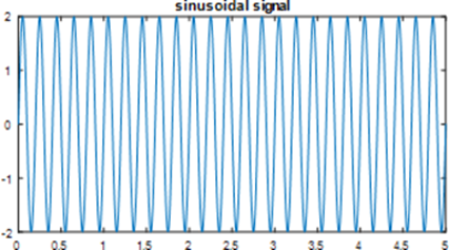
Figure 2. Original sinusoidal Signals.

Download: Download full-size image

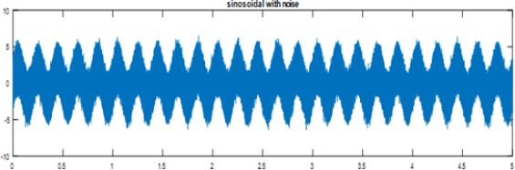
Figure 3. Simulation result of sinusoidal signal with noise.

The above figures 2 and 3 simulation result plots shows that figure 2 the input sinusoidal signal and figure 3 the sinusoidal signal with noise with different environmental and materials noise sources destructed.

Download: Download full-size image

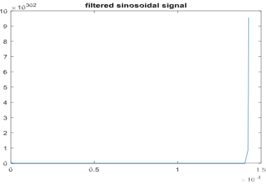
Figure 4. Filtered sinusoidal signal.

The above Figure 4 simulation results describes the filtered sinusoidal signal that the noise signal is filtered by using FIR and IIR filtering techniques. The Figure 4 shows that the filter at is at 0 frequency level and after some times the signal frequency increasing continuously. That filters avoids the unwanted signals or noisy signals and that to get the desired signals. The reason to filter the signals to reduce and smooth out the high frequency noise associated with a measurement. High frequency noise normally considered random and additive to a measured signal. The reason to filter a signal is to reduce and smooth out high-Frequency noise associated with a measurement.

Download: Download full-size image

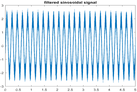
Figure 5. Filtered sinusoidal signal.

The above Figure 5 shows that the goal of the filtering of signals from noise by using finite impulse response (FIR) technique and it is the final result of the signal that is filtered signal mean that extracted signal or the desired signal we get by removing the noisy signal/unwanted signal.

3.2. LMS Filter for Noise Cancellation

The post-processing LMS filter designed using Simulink, MATLAB 2017a. The algorithm computes the filtered output, error and the filter weights for a given input and desired signal using the Least Mean Squares (LMS) algorithm. The LMS filter used to identify an FIR signal embedded in noise.

Download: Download full-size image

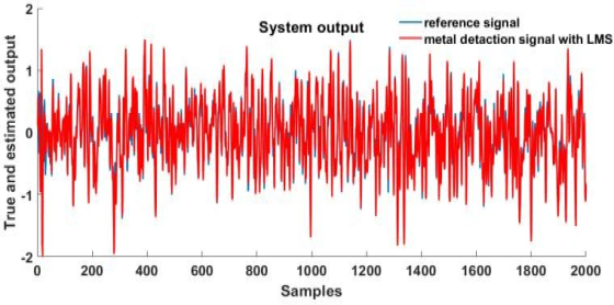
Figure 6. Outputs with Least Mean Square (LMS) filtering technique.

The simulation result is the Adaptive noise canceller Simulink Model scope output. In this, the waveform is represents output signal entering into the system. On the above figure 6, the LMS filter is an adaptive filter that adjusts its filter coefficients iteratively to minimize the mean square error between the output signal and the desired signal. It uses a gradient-based approach to update the filter coefficients, making it a type of stochastic gradient descent algorithm.

Download: Download full-size image

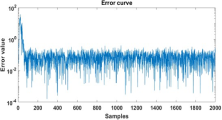
Figure 7. Errors with LMS.

The simulation results of the noise cancellation with LMS Filter as well as the proposed technique error signal shown in figure 7. The variation of error signal after filtration varies Between a maximum of -1 to +1 which is well inside the limits to be considered. The error signal, which defined by the difference of desired signal and input signal.

Download: Download full-size image

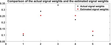
Figure 8. Comparisons of actual signal weights and the estimated signal weights.

3.3. System Identification of FIR Filter Using LMS Algorithm

System identification is the process of identifying the coefficients of an unknown system using an adaptive filter. The general overview of the process shown in Figure 9.

With the unknown filter designed and the desired signal in place, create and apply the adaptive LMS filter object to identify the unknown filter. Preparing the adaptive filter object requires starting values for estimates of the filter coefficients and the LMS step size (mu). Starting with some set of nonzero values as estimates for the filter coefficients. This plot uses zeros for the 13 initial filter weights. Set the Initial Conditions property of DSP. LMS filter to the desired initial values of the filter weights. For the step size, 0.8 is a good compromise between being large enough to converge well within 250 iterations (250 input sample points) and small enough to create an accurate estimate of the unknown filter.

Download: Download full-size image

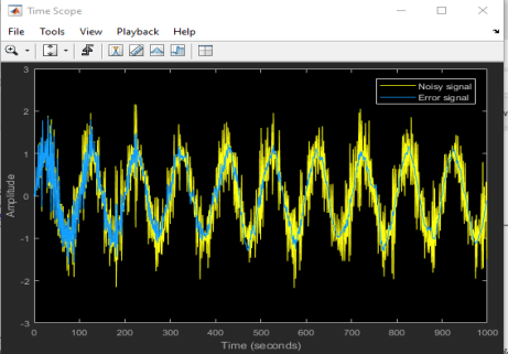
Figure 9. Simulation results of noisy signal and error signal based on system identification.

Download: Download full-size image

Figure 10. Simulation results of comparison of Weight.

The above figure 10 shows the System Identification is the process of determining the attributes of the system by repetitive experimentation. Here, the system examined is a Finite Impulse Response (FIR) filter. If the Impulse response of a system is having finite number of coefficients such a system is called finite impulse response filter.

3.4. Experimental Results

Two samples one without crack and other with crack were tested using the UFD-01/T flaw detector. The FFT spectrum of the sample free crack is displayed Figures 11, 12 and 13 shown the snapshots of the FFT spectrum for the cracked sample, which was influenced by environmental noise such as welding and acoustic noises. Due to the lack of a bus interface on the UFD-01/T, extracting raw data directly was challenging. To enable further post processing and filtering, the FFT snapshot were converted in to a raw data file using third party software called “Get data graph digitizer”. The experimental pulse-echo signals were obtained using a circle ultrasonic probe longitudinal wave 6 MHz of center frequency and 10 mm in diameter. Sampling frequency is 12MHz.

As illustrated in Figure 11, the transmission signal is primarily centered approximately 0.7MHz. The back wall echo appears around 1MHz, while the surface echo is centered near 1.3MHz. A peak observed at about 1.5 MHZ is attributed to grain structure and unwanted noise, with a signal strength close -23dBm, representing the noise floor for the crack free sample. Additionally, spurious signals above 1.5 MHz correspond to higher order frequency components.

Download: Download full-size image

Figure 11. Experimental result of standard welded sample 1 without noise.

Download: Download full-size image

Figure 12. Experimental results 2 sample without defect with welding noise.

As shown in the above figure 12 the transmission signal is centered around 0.7MHz, back wall echo is centered around 1MHz, at the surface echo is centered around 1.3MHz, around 1.5 MHZ peaking is due to grain structure and unwanted noise and that signal strength is around -23dBm, which is the noise floor of the sample without crack. The spurs greater than 1.5 MHz are due to higher order frequency components.

In the above figure 4 the experimental result shows the corrupted or disturbed signals with the noise of the nearest running induction motor and vibration noise. However, without noise, the crack detected at 2.4MHz. to delineate the flaw frequency from the noisy environment, the FIR and IIR filters were designed using Filter design toolbox of MATLAB and the time domain and frequency domain results are populated in the following section.

Download: Download full-size image

Figure 13. Experimental results 3 with running induction motor noise.

3.5 Simulation Results

The parameters examined in this study include sampling frequency, cutoff frequency, time duration (period), signal frequency, passband frequency, stopband frequency, passband attenuation, and stopband attenuation. As shown in Figure 14, a signal with a sampling frequency of 6 MHz was applied to the metal, producing sinusoidal waves. These waves indicate that the signal effectively propagates through the metal, allowing for direct measurement of the crack location, back wall echo, and the material’s surface. The propagation time corresponds to the range of the signal’s reflections; a longer propagation time suggests the absence of cracks. Moreover, the presence of back wall echo and surface reflections confirms normal conditions, indicating that the material is free of cracks.

Download: Download full-size image

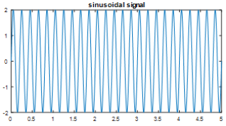
Figure 14. Original sinusoidal Signals.

Download: Download full-size image

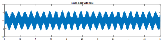
Figure 15. Simulation result of sinusoidal signal with noise.

The simulation results presented in Figure 15 indicate that the signal is distorted by external noise sources. These noise contributors—including the material’s grain structure, transducer distance, overlapping test materials, and electronic circuitry—are inherent challenges during metal testing. For accurate detection, it is crucial to separate unwanted noise from the desired signals. However, noise removal remains difficult even with advanced, well-calibrated instruments. To address this, various filtering techniques, such as FIR and IIR filters, will be applied to eliminate undesired signals. In Figure 15, the horizontal axis represents time duration in microseconds (µs), while the vertical axis shows amplitude in decibels (dB), illustrating the simulation results..

Download: Download full-size image

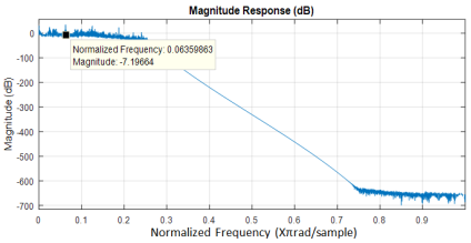
Figure 16. Simulation result of magnitude response.

The simulation results shown in Figure 16 depict the magnitude on the y-axis in decibels (dB) and the normalized frequency on the x-axis in terms of *π radians per sample. From the graph, it is observed that the magnitude of the metal during the conversion of sound energy to electrical energy is zero at certain points, indicating no sound occurrence. However, at some instances, both positive and negative magnitudes appear. Positive values indicate that the sound is louder than the threshold or has a faster response than the threshold, while negative values indicate that the sound is softer or has a slower response than the threshold. Over time, the sound magnitude decays linearly, showing that the sound response slows down more quickly than the threshold. Beyond 0.75 rad/sample, the sound response becomes entirely negative, reaching approximately -650 dB, which means the sound pressure level is significantly below the threshold.

The simulation results shown in Figure 17 illustrate the filtered sinusoidal signal after applying FIR and IIR filtering techniques to remove noise. The figure shows that the filter starts at a frequency level of 0, and the signal frequency increases steadily over time. These filters effectively eliminate unwanted or noisy signals, allowing the desired signals to be obtained. The primary purpose of filtering is to reduce and smooth out high-frequency noise, which is typically random and additive to the measured signal. By filtering, the measurement becomes clearer and more accurate.

Download: Download full-size image

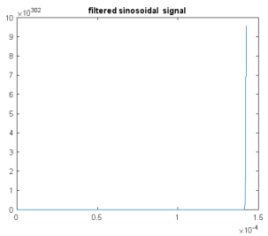
Figure 17. Simulation result of filtered sinusoidal signal.

Download: Download full-size image

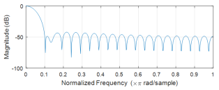
Figure 18. Simulation result of magnitude response.

Figure 18 shows the magnitude response simulation results, where the y-axis represents magnitude in decibels (dB) and the x-axis represents normalized frequency (*π radians/sample). The graph demonstrates that the FIR filter, which acts as a low-pass filter, allows low-frequency signals to pass while attenuating high-frequency signals. Low-pass filters are commonly used to remove high-frequency noise from input signals. Since noise typically consists of high-frequency components, passing the signal through a low-pass filter effectively reduces noise and produces a clearer sound. The cutoff frequency in this result corresponds to a magnitude of -50 dB; frequencies with magnitudes below this threshold are filtered out, meaning high-frequency noise is removed while lower-frequency signals are preserved.

Download: Download full-size image

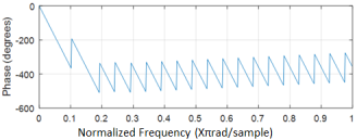
Figure 19. Simulation result of phase response.

Figure 19 illustrates the phase response, with the y-axis representing phase in degrees and the x-axis showing normalized frequency (*π radians/sample). As expected from a low-pass FIR filter, low-frequency signals pass through while high-frequency signals are attenuated. Unlike an ideal filter, this designed filter exhibits a smoother transition between the passband and stopband. Additionally, some ripples are present in both bands. Low-pass filters are commonly used to remove high-frequency noise from input signals, resulting in a clearer output. The cutoff frequency corresponds to a phase response below -200 degrees; beyond this point, phase ripples caused by the filter’s non-linear phase response can distort the waveform. The magnitude response of the rectangular window, as shown in Figure 19, explains these ripples and ringing effects introduced in the FIR filter response.

Figure 20 illustrates the outcome of filtering signals using the Finite Impulse Response (FIR) technique. The figure represents the final filtered signal, which is the desired signal obtained after removing unwanted noise and interference.

An IIR filter provides the advantage of achieving a roll-off comparable to that of an FIR filter but with a lower order, meaning it requires fewer terms. This leads to reduced computational effort and faster processing speeds. However, IIR filters may exhibit nonlinear phase responses and potential stability issues. This scenario is akin to the fable of the tortoise and the hare: the FIR filter resembles the tortoise slow, steady, and reliable consistently finishing the race. In contrast, the IIR filter is like the hare fast and efficient but occasionally prone to instability and failure to complete the task.

Download: Download full-size image

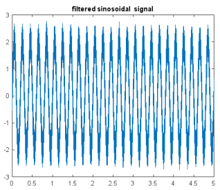
Figure 20. Simulation result of filtered sinusoidal signal.

4. Conclusions

One of the fundamental challenges affecting the performance of testing materials with nondestructive testing by ultrasonic NDT method is the undesired impact of noise on a signal. Noise can distort the true signal and arise from several sources, including system non-linearity and noise interference from adjacent environment. Conventional communication systems use filters to cancel noise in a received signal. In the case of ultrasonic NDT systems, noise cancellation of a signal is important during the materials testing time; the results, both FIR and IIR filtering techniques have been effectively applied to cancellation noisy signal in ultrasonic signal. An adaptive noise cancellation system was successfully simulated and implemented, achieving the required signal to noise floor performance. The ultrasonic data was effectively filtered, allowing the noisy signals data to be sufficiently filtered to recover the target signal. Simulation results demonstrated that the noise level was reduced by more than 20 dBm, and the resolution improved by a factor of two when using the adaptive filtering algorithm. However, some challenges were encountered during the Signal analysis with the ultrasonic equipment. Specifically, transferring raw data files into MATLAB proved difficult due to the lack of dedicated software for interfacing the NDT device with the computer.

Abbreviations

NDE	Non-Destructive Evaluation
NDT	Non-Destructive Testing
UFD	Ultrasonic Flaw Detection
FFT	Fast Fourier Transform
FIR	Finite Impulse Response
IIR	Infinite Impulse Response
LMS	Least Mean Square
FPGA	Ultrasonic Signal Processing Platform
RTL	Register Transfer Level
DLMS	Delayed Least Mean Square
RLS	Recursive Least Squares
NLMS	Normalized Least Mean Square
BMI	Body Mass Index
UV	Ultraviolet
HV	Vickers Hardness
HS	Shrinkage According Height
DS	Shrinkage According Diameter

Acknowledgments

The authors expresses gratitude to Dr. Ramasamy Srinivasagan and Dr. Sairoel Amertet for his constructive comments and suggestions throughout the research. We extendedly acknowledge to the Metals Industry Development Institute of Ethiopian for its comprehensive sponsorship and logistical support during fieldwork.

Author Contributions

Birtukan Yenealem: Conceived and designed the experiments; Performed the experiments; Analyzed and interpreted the data; Contributed reagents, materials, analysis tools or data; Wrote the paper

Mamaru Genetu: Analyzed and interpreted the data; Contributed reagents, analysis data; editing, wrote the paper

Elias Mamushet: Analyzed and interpreted the data; Contributed reagents, analysis data; wrote the paper

Availability of Data

The data used in the study will be available upon request.

Conflicts of Interest

The authors declare no conflicts of interest.

References

[1]	G. V. P. Chandra, S. Yadav, B. A. Krishna, and M. Kamaraju, “Performance of Wiener Filter and Adaptive Filter for Noise Cancellation in Real-Time Environment,” Int. J. Comput. Appl., vol. 97, no. 15, 2014.
[2]	B. A. Krishna and G. C. S. Yadav, “Performance Comparison of Different Variable Filters for Noise Cancellation in Real-Time Environment,” Int. J. Signal Process. Image Process. Pattern Recognit., vol. 9, no. 2, pp. 107-126, 2016.
[3]	G. C. S. Yadav and B. A. Krishna, “Study of different adaptive filter algorithms for noise cancellation in real-Time environment,” Int. J. Comput. Appl., vol. 96, no. 10, 2014.
[4]	Y.-H. Chen, S.-J. Ruan, and T. Qi, “An automotive application of real-time adaptive wiener filter for non-stationary noise cancellation in a car environment,” in 2012 IEEE International Conference on Signal Processing, Communication and Computing (ICSPCC 2012), 2012, pp. 597-601. https://doi.org/10.1109/ICSPCC.2012.6335671
[5]	H. Kaur and R. Talwar, “Performance and convergence analysis of LMS algorithm,” in 2012 IEEE International Conference on Computational Intelligence and Computing Research, 2012, pp. 1-4. https://doi.org/10.1109/ICCIC.2012.6510264
[6]	H.-C. Huang and J. Lee, “A new variable step-size NLMS algorithm and its performance analysis,” IEEE Trans. Signal Process., vol. 60, no. 4, pp. 2055-2060, 2011. https://doi.org/10.1109/TSP.2011.2172407
[7]	C. Brady, J. Arbona, I. S. Ahn, and Y. Lu, “FPGA-based adaptive noise cancellation for ultrasonic NDE application,” in 2012 IEEE International Conference on Electro/Information Technology, 2012, pp. 1-5. https://doi.org/10.1109/EIT.2012.6220702
[8]	R. Jose and M. Brindha, “Area Optimized Adaptive Noise Cancellation System Using FPGA for Ultrasonic NDE Applications: A Design and Simulation Approach,” Signal Process., vol. 5, p. 11.
[9]	U. Meyer-Baese and U. Meyer-Baese, Digital signal processing with field programmable gate arrays, vol. 65. Springer, 2007. https://doi.org/10.1007/978-3-540-72613-3
[10]	K. A. Tiwari, R. Raisutis, and V. Samaitis, “Signal processing methods to improve the Signal-to-noise ratio (SNR) in ultrasonic non-destructive testing of wind turbine blade,” Procedia Struct. Integr., vol. 5, pp. 1184-1191, 2017. https://doi.org/10.1016/j.prostr.2017.07.134
[11]	R. Drai, F. Sellidj, M. Khelil, and A. Benchaala, “Elaboration of some signal processing algorithms in ultrasonic techniques: application to materials NDT,” Ultrasonics, vol. 38, no. 1-8, pp. 503-507, 2000.
[12]	K. A. Tiwari, A. Ostreika, and J. Platuziene, “Efficient FPGA-based FIR- architecture and its significance in ultrasonic signal processing,” J. Vibroengineering, vol. 19, no. 8, pp. 6423-6432, 2017.
[13]	J. E. González, E. F. Forero, and D. A. Tibaduiza, “Signal Denoising by Using Adaptive Filtering in Signals from Ultrasonic Sensors.”
[14]	M. Li and G. Hayward, “A robust approach to optimal matched filter design in ultrasonic non-destructive evaluation (NDE),” in AIP Conference Proceedings, 2017, vol. 1806, no. 1, p. 140002. https://doi.org/10.1063/1.4974636
[15]	P. M. Shankar, P. Karpur, V. L. Newhouse, and J. L. Rose, “Split-spectrum processing: Analysis of polarity threshold algorithm for improvement of signal-to-noise ratio and detectability in ultrasonic signals,” IEEE Trans. Ultrason. Ferroelectr. Freq. Control, vol. 36, no. 1, pp. 101-108, 1989. https://doi.org/10.1109/58.20283
[16]	R. Mallett, P. J. Mudge, T. H. Gan, and W. Balachandra, “Analysis of cross- correlation and wavelet de-noising for the reduction of the effects of dispersion in long- range ultrasonic testing,” Insight-Non-Destr. Test. Cond. Monit., vol. 49, no. 6, pp. 350- 355, 2007. https://doi.org/10.1784/insi.2007.49.6.350
[17]	S. Iyer, S. K. Sinha, B. R. Tittmann, and M. K. Pedrick, “Ultrasonic signal processing methods for detection of defects in concrete pipes,” Autom. Constr., vol. 22, pp. 135-148, 2012. https://doi.org/10.1016/j.autcon.2011.06.008
[18]	Vengrinovich, V. (2013) New Trends in Non-Destructive Evaluation of Surface Hardened Layers and Coatings. Journal of Surface Engineered Materials and Advanced Technology, 3, 154-162. https://doi.org/10.4236/jsemat.2013.32020
[19]	Karaseva, V., Lvov, A. and Rodionov, A. (2023) Frequency-Domain Wideband Acoustic Noise Cancellation System. Journal of Applied Mathematics and Physics, 11, 2523-2532. https://doi.org/10.4236/jamp.2023.118163

Cite This Article

Plain Text BibTeX RIS

APA Style

Yenealem, B., Genetu, M., Mamushet, E. (2025). Applications of Adaptive Filtering Techniques for Noise Cancellation Systems to the Ultrasonic Non-Destructive Evaluation (NDE). Journal of Electrical and Electronic Engineering, 13(4), 168-183. https://doi.org/10.11648/j.jeee.20251304.13

Copy | Download

ACS Style

Yenealem, B.; Genetu, M.; Mamushet, E. Applications of Adaptive Filtering Techniques for Noise Cancellation Systems to the Ultrasonic Non-Destructive Evaluation (NDE). J. Electr. Electron. Eng. 2025, 13(4), 168-183. doi: 10.11648/j.jeee.20251304.13

Copy | Download

AMA Style

Yenealem B, Genetu M, Mamushet E. Applications of Adaptive Filtering Techniques for Noise Cancellation Systems to the Ultrasonic Non-Destructive Evaluation (NDE). J Electr Electron Eng. 2025;13(4):168-183. doi: 10.11648/j.jeee.20251304.13

Copy | Download

@article{10.11648/j.jeee.20251304.13,
  author = {Birtukan Yenealem and Mamaru Genetu and Elias Mamushet},
  title = {Applications of Adaptive Filtering Techniques for Noise Cancellation Systems to the Ultrasonic Non-Destructive Evaluation (NDE)
},
  journal = {Journal of Electrical and Electronic Engineering},
  volume = {13},
  number = {4},
  pages = {168-183},
  doi = {10.11648/j.jeee.20251304.13},
  url = {https://doi.org/10.11648/j.jeee.20251304.13},
  eprint = {https://article.sciencepublishinggroup.com/pdf/10.11648.j.jeee.20251304.13},
  abstract = {The performance of ultrasonic non-destructive evaluation (NDE) systems is frequently limited by backscattering and electronic noise, which reduce sensitivity and resolution, particularly in industrial environments. At the Metals Industry Development Institute in Ethiopia, the ultrasonic NDT flaw detector (model UFD-01/T) has been employed to defects internal material defects. However, accurately pinpointing crack related frequencies remains difficult due to substantial environmental noise interference. To address this challenge, a post-processing noise cancellation system was developed utilizing advanced adaptive filtering techniques. This study presents mathematical models for noise reduction and evaluates the effectiveness of several adaptive filter algorithms, including Fast Fourier Transform (FFT), Finite Impulse Response (FIR), Infinite Impulse Response (IIR), and Least Mean Square (LMS) methods. These algorithms were implemented and simulated within the MATLAB environment to assess their ability to isolate defect signals from noise. Simulation results demonstrate that the proposed adaptive filtering methods, particularly the LMS algorithm, effectively attenuate high-frequency noise originating from echoes and environmental interferences. Consequently, the noise floor in the processed ultrasonic signals was reduced to below 35 dBm, significantly enhancing the capability to localize material defects. These findings support the integration of adaptive filtering techniques in ultrasonic NDE systems to improve defect detection precision in noisy industrial environments, thereby enhancing inspection reliability, reducing false positives, and contributing to the overall safety and efficiency of industrial operations.},
 year = {2025}
}

Copy | Download

TY  - JOUR
T1  - Applications of Adaptive Filtering Techniques for Noise Cancellation Systems to the Ultrasonic Non-Destructive Evaluation (NDE)

AU  - Birtukan Yenealem
AU  - Mamaru Genetu
AU  - Elias Mamushet
Y1  - 2025/07/28
PY  - 2025
N1  - https://doi.org/10.11648/j.jeee.20251304.13
DO  - 10.11648/j.jeee.20251304.13
T2  - Journal of Electrical and Electronic Engineering
JF  - Journal of Electrical and Electronic Engineering
JO  - Journal of Electrical and Electronic Engineering
SP  - 168
EP  - 183
PB  - Science Publishing Group
SN  - 2329-1605
UR  - https://doi.org/10.11648/j.jeee.20251304.13
AB  - The performance of ultrasonic non-destructive evaluation (NDE) systems is frequently limited by backscattering and electronic noise, which reduce sensitivity and resolution, particularly in industrial environments. At the Metals Industry Development Institute in Ethiopia, the ultrasonic NDT flaw detector (model UFD-01/T) has been employed to defects internal material defects. However, accurately pinpointing crack related frequencies remains difficult due to substantial environmental noise interference. To address this challenge, a post-processing noise cancellation system was developed utilizing advanced adaptive filtering techniques. This study presents mathematical models for noise reduction and evaluates the effectiveness of several adaptive filter algorithms, including Fast Fourier Transform (FFT), Finite Impulse Response (FIR), Infinite Impulse Response (IIR), and Least Mean Square (LMS) methods. These algorithms were implemented and simulated within the MATLAB environment to assess their ability to isolate defect signals from noise. Simulation results demonstrate that the proposed adaptive filtering methods, particularly the LMS algorithm, effectively attenuate high-frequency noise originating from echoes and environmental interferences. Consequently, the noise floor in the processed ultrasonic signals was reduced to below 35 dBm, significantly enhancing the capability to localize material defects. These findings support the integration of adaptive filtering techniques in ultrasonic NDE systems to improve defect detection precision in noisy industrial environments, thereby enhancing inspection reliability, reducing false positives, and contributing to the overall safety and efficiency of industrial operations.
VL  - 13
IS  - 4
ER  -

Copy | Download

Author Information

Birtukan Yenealem

Minerals Industry Development Institute, Ministry of Mines, Addis Ababa, Ethiopia. Department of Electromechanical Engineering, Addis Ababa Science and Technology University, Addis Ababa, Ethiopia

Contact Email

http://orcid.org/0009-0004-9728-0324
Mamaru Genetu

Minerals Industry Development Institute, Ministry of Mines, Addis Ababa, Ethiopia

Contact Email

http://orcid.org/0000-0002-1406-3032
Elias Mamushet

Department of Mining Engineering, Addis Ababa Science and Technology University, Addis Ababa, Ethiopia

http://orcid.org/0009-0002-6159-1003

Download PDF

Submit an Article

Plain Text BibTeX RIS

APA Style

Yenealem, B., Genetu, M., Mamushet, E. (2025). Applications of Adaptive Filtering Techniques for Noise Cancellation Systems to the Ultrasonic Non-Destructive Evaluation (NDE). Journal of Electrical and Electronic Engineering, 13(4), 168-183. https://doi.org/10.11648/j.jeee.20251304.13

Copy | Download

ACS Style

Yenealem, B.; Genetu, M.; Mamushet, E. Applications of Adaptive Filtering Techniques for Noise Cancellation Systems to the Ultrasonic Non-Destructive Evaluation (NDE). J. Electr. Electron. Eng. 2025, 13(4), 168-183. doi: 10.11648/j.jeee.20251304.13

Copy | Download

AMA Style

Yenealem B, Genetu M, Mamushet E. Applications of Adaptive Filtering Techniques for Noise Cancellation Systems to the Ultrasonic Non-Destructive Evaluation (NDE). J Electr Electron Eng. 2025;13(4):168-183. doi: 10.11648/j.jeee.20251304.13

Copy | Download

@article{10.11648/j.jeee.20251304.13,
  author = {Birtukan Yenealem and Mamaru Genetu and Elias Mamushet},
  title = {Applications of Adaptive Filtering Techniques for Noise Cancellation Systems to the Ultrasonic Non-Destructive Evaluation (NDE)
},
  journal = {Journal of Electrical and Electronic Engineering},
  volume = {13},
  number = {4},
  pages = {168-183},
  doi = {10.11648/j.jeee.20251304.13},
  url = {https://doi.org/10.11648/j.jeee.20251304.13},
  eprint = {https://article.sciencepublishinggroup.com/pdf/10.11648.j.jeee.20251304.13},
  abstract = {The performance of ultrasonic non-destructive evaluation (NDE) systems is frequently limited by backscattering and electronic noise, which reduce sensitivity and resolution, particularly in industrial environments. At the Metals Industry Development Institute in Ethiopia, the ultrasonic NDT flaw detector (model UFD-01/T) has been employed to defects internal material defects. However, accurately pinpointing crack related frequencies remains difficult due to substantial environmental noise interference. To address this challenge, a post-processing noise cancellation system was developed utilizing advanced adaptive filtering techniques. This study presents mathematical models for noise reduction and evaluates the effectiveness of several adaptive filter algorithms, including Fast Fourier Transform (FFT), Finite Impulse Response (FIR), Infinite Impulse Response (IIR), and Least Mean Square (LMS) methods. These algorithms were implemented and simulated within the MATLAB environment to assess their ability to isolate defect signals from noise. Simulation results demonstrate that the proposed adaptive filtering methods, particularly the LMS algorithm, effectively attenuate high-frequency noise originating from echoes and environmental interferences. Consequently, the noise floor in the processed ultrasonic signals was reduced to below 35 dBm, significantly enhancing the capability to localize material defects. These findings support the integration of adaptive filtering techniques in ultrasonic NDE systems to improve defect detection precision in noisy industrial environments, thereby enhancing inspection reliability, reducing false positives, and contributing to the overall safety and efficiency of industrial operations.},
 year = {2025}
}

Copy | Download

TY  - JOUR
T1  - Applications of Adaptive Filtering Techniques for Noise Cancellation Systems to the Ultrasonic Non-Destructive Evaluation (NDE)

AU  - Birtukan Yenealem
AU  - Mamaru Genetu
AU  - Elias Mamushet
Y1  - 2025/07/28
PY  - 2025
N1  - https://doi.org/10.11648/j.jeee.20251304.13
DO  - 10.11648/j.jeee.20251304.13
T2  - Journal of Electrical and Electronic Engineering
JF  - Journal of Electrical and Electronic Engineering
JO  - Journal of Electrical and Electronic Engineering
SP  - 168
EP  - 183
PB  - Science Publishing Group
SN  - 2329-1605
UR  - https://doi.org/10.11648/j.jeee.20251304.13
AB  - The performance of ultrasonic non-destructive evaluation (NDE) systems is frequently limited by backscattering and electronic noise, which reduce sensitivity and resolution, particularly in industrial environments. At the Metals Industry Development Institute in Ethiopia, the ultrasonic NDT flaw detector (model UFD-01/T) has been employed to defects internal material defects. However, accurately pinpointing crack related frequencies remains difficult due to substantial environmental noise interference. To address this challenge, a post-processing noise cancellation system was developed utilizing advanced adaptive filtering techniques. This study presents mathematical models for noise reduction and evaluates the effectiveness of several adaptive filter algorithms, including Fast Fourier Transform (FFT), Finite Impulse Response (FIR), Infinite Impulse Response (IIR), and Least Mean Square (LMS) methods. These algorithms were implemented and simulated within the MATLAB environment to assess their ability to isolate defect signals from noise. Simulation results demonstrate that the proposed adaptive filtering methods, particularly the LMS algorithm, effectively attenuate high-frequency noise originating from echoes and environmental interferences. Consequently, the noise floor in the processed ultrasonic signals was reduced to below 35 dBm, significantly enhancing the capability to localize material defects. These findings support the integration of adaptive filtering techniques in ultrasonic NDE systems to improve defect detection precision in noisy industrial environments, thereby enhancing inspection reliability, reducing false positives, and contributing to the overall safety and efficiency of industrial operations.
VL  - 13
IS  - 4
ER  -

Copy | Download