Research Article | | Peer-Reviewed

Optimizing Staffing for a New Medical Facility

Received: 18 March 2026     Accepted: 1 April 2026     Published: 16 April 2026
Views:       Downloads:
Abstract

When a new medical facility is planned, there is a need for staff members of various job roles and levels. For each of these roles, there are several different classifications for staff. Each of these classification groups have their respective advantages and disadvantages in terms of cost, productivity, new ideas, and other characteristics. Some of these characteristics have a continuous range of values, which differ for each type of job role. In addition, there are boundary conditions characteristics, which only have binary values (True/False), that also limit the proportion for each classification group. While the number of classifications is not limited, this publication will consider examples with three primary classifications for staff: early career hires, experienced hires, and (experienced) transfers. This article details a method for using these metrics and boundary conditions to optimize the staffing using a visualization approach. While the equations for the metrics and boundary conditions can be solved directly and we show how that can be done, they do not answer how the optimum solution is obtained in the way that visualizations can. Since each facility and location may have its own unique requirements, this article discusses general principles and mathematical processes rather than exact prescriptions.

Published in Journal of Human Resource Management (Volume 14, Issue 2)
DOI 10.11648/j.jhrm.20261402.15
Page(s) 144-157
Creative Commons

This is an Open Access article, distributed under the terms of the Creative Commons Attribution 4.0 International License (http://creativecommons.org/licenses/by/4.0/), which permits unrestricted use, distribution and reproduction in any medium or format, provided the original work is properly cited.

Copyright

Copyright © The Author(s), 2026. Published by Science Publishing Group

Keywords

Staffing, New Facility, Early Career, Experienced Career, Transfers, Staff Reductions, Facility Expansion

1. Introduction
When a new medical facility is planned, a large number of staff are needed from a variety of job families. The specifics are based on HR policies with associated costs in terms of salaries and effectiveness . The staffing levels of a new or expanded facility in terms of Nursing , Allied Health , skills mix , and even Pastoral Care have been extensively reported. What has not been examined is how to maximize a series of metrics consistent with a set of boundary conditions during this staffing process. The metrics can include maximizing productivity and experience while minimizing cost and inefficiency and imposing boundary conditions that can ensure there is sufficient staff to serve as mentors for junior employees. This point in the hiring space will be referred to as the “Hiring Sweet Spot”. This publication will examine the process to determine the “Hiring Sweet Spot” using a reduced set of classifications that lend themselves to a 2-dimenstional visualization. However, the process is not dependent on the visualizations and additional classifications, which make the overall hiring space more difficult to visualize, can be included without a significant change in the process or a loss of its effectiveness. As the hiring process evolves, future hiring will need to shift from the “Hiring Sweet Spot” in such a way that the sum of current and future hires will leave the final facility hiring at the most effective point in the hiring space. Several examples of each of these steps, along with the underlying mathematics, will be discussed in detail.
Within each job-family, there are different classifications of employees. The number of classifications will dictate the geometry of the visualization that is required. Two classifications lead to a line (or a rectangle to make the gradients clearer), three classifications can be shown in a triangle, four classifications would be a 3-dimensional tetrahedron, and five or more classifications would be a multi-dimensional equilateral polygon. Since multi-dimensional figures are difficult to visualize on a 2-dimensional page, the three classifications figure of a triangle will be used herein with an experienced hire, an early career hire, and a transfer from another location within the organization being the three classifications.
This article details a method to optimize staffing based on a desired set of metrics, such as productivity, cost, market availability, and effectiveness. In addition, there are other limiting boundary conditions, such as having sufficient experienced staff to daily mentor junior staff and the desire to have a mixture of the different classifications that are necessary considerations in the hiring process. The choices for metrics and boundary conditions are almost limitless; however, since each healthcare facility has its own unique requirements and non-medical facilities have even more different requirements, this article discusses general principles and mathematical processes that can be applied to determine an optimum staffing mix regardless of the industry or jobs.
2. Materials and Methods
2.1. Triangle Coordinate System
In this paper, three classifications will be examined as an equilateral triangle to represent the space of possible combinations of the triplet (Early Career Hire, Experienced Hire, Transfer) percentages, see Figure 1. The coordinate system in the triangle used to designate the boundary conditions and the metrics is based on the work of Nagy and Abuhmaidan .
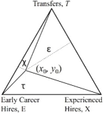
Figure 1. Equilateral Triangle graphical representation of an (Early Career, Experienced Career, Transfer) triplet.
Since these percentages must total 100%, only two of the values are truly independent with the other being dependent on the two independent variables. While the choice of the dependent variable and the independent variables is immaterial, there is a reason, that will be discussed later, to not have Transfers as the dependent variable. Therefore, Transfers, T, and Experienced, X, are designated as the independent values, which leaves the Early Career, E, as the dependent variable with a value of:
E=1-T -X(1)
The percentage of each of these triplet components is determined by the area of the sub-triangle located opposite the vertex of the part of the triplet as shown in Figure 1. The area of any triangle can be calculated using the “Surveyor's Area Formula", discussed by Braden , from the coordinates of its three vertices, (x1, y1), (x2, y2), and (x3, y3):
Triangle Area= 12 111x1x2x3y1y2y3 (2)
=12x1y2-y3+x2y3-y1+x3(y1-y2)
If the three vertices are labeled in a counterclockwise sequence, the absolute value is not needed. That assumption will be used moving forward.
For an equilateral triangle with a side length of 1, the height and area of the triangle are 32/2 and 32/4, respectively. For the entire triangle and the three sub-triangles in Figure 1, the coordinates of the three outer vertices and an arbitrary internal point (x0, y0), are shown in Table 1.
Table 1. Vertices of Triangle in Figure 1.

Vertex

X

Y

Early Career Hire

0.0

0.0

Experienced Hire

1.0

0.0

Transfer

0.5

32/2

Interior Point

X0

Y0

The area of any triangle is
Area=Base (Height)2(3)
In an equilateral triangle, the length of the base is the same, so the areas are simply proportional to the triangle heights ε, χ, and τ, respectively in Figure 1 and are calculated using the formulas by Ballantine and Jerbert where the distance from a line is defined by (x1, y1) and (x2, y2) and the point of interest is (x0, y0):
x0y2- y1- y0x2- x1+ x2y1-x1y2y2- y12+x2- x12 2(4)
For these triangles, the lines are sides of the main triangle connecting the vertices as shown in Figure 1 and Table 1. The denominator of this equation is the length of the sides of the main triangle, which, in this case, is 1 for all of the sub-triangles. (Remember, these vertices in this equation are the ones opposite the vertex being calculated, that is for Experienced Hires, the Early Career Hire, and Transfers vertices are needed along with the interior point of interest.)
Using the equations (2), (3), and (4), it is straight forward to go from a point inside the triangle to the corresponding triplet and from a triplet to the corresponding point inside the triangle. For an arbitrary point, (x0, y0), in Figure 1, the corresponding triangle heights ε, χ, and τ, areas, and relative areas are shown in Table 2. From this table, the previous statement about τ being an obvious choice as one of the independent variables is clear. In addition, the totals for each column are 32/2, 32/4, and 1, as expected.
Table 2. Height, Area, and Relative Areas of the Sub-Triangles in Figure 1.

Vertex

Height

Area

Relative Area

Early Career Hire, ε

123 2- 3 2x0- y0

143 2- 3 2x0- y0

(1- x0)- 3 23y0

Experienced Hire, χ

123 2x0- y0

143 2 x0- Yy0

 x0- 3 23y0

Transfer, τ

y0

12y0

2 323y0

Totals

3 22

3 24

1

For the triplet (Early Career Hire, Experienced Hire, Transfer) of (ε, χ, τ), the position of the corresponding point (x0, y0), is
y0= 3 22 τ(5)
x0= χ+ 39 τ
In Figure 1, the point in question is (63%, 9%, 28%) and the coordinates are (0.183, 0.242).
2.2. Metrics and Boundary Conditions Graphs
The various metrics and boundary conditions will be shown as triangles of levels of grey and black and white, respectively, as shown in Figure 2. The darker the shading shows the hiring triplet regions that should be avoided while the lighter shading shows more favorable hiring triplet values based on the combination of the Metrics and Boundary Conditions.
The white/black transition of a boundary condition is the extreme of the favorable/unfavorable scale and can be viewed as a “Yes” / “No” binary value, respectively. While the choice of black or white for the favorable and unfavorable regions is arbitrary, the selection of black as unfavorable has the mathematical advantage of being zero and, when multiplied by anything else, would always be zero. Similarly, white being one on the gray scale, leaves anything multiplied by it unchanged.
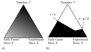
Figure 2. Graphical representation of a Metric such as experience or salary (a, left) and a Boundary Condition requiring sufficient mentors (b, right).
As a Metric example, Figure 2a shows the triangle where Early Career Hires, Experienced Hires, and Transfers have a ratio for some metric, such as experience or salary, of 20%, 40%, and 90%, respectively. A boundary condition that requires at least one Transfer for each Early Career Hire and a Transfer for each three Experienced Hires, would be represented like Figure 2b.
These triangles are easily produced in R or other graphic capable languages or applications. (The R script used for all the calculations and images in this section (for Figures 2 and 3) is included in the Appendix. It is designed to be modular and is easily modified or expanded.)
2.3. Composite Metric Triangles and Composite Boundary Condition Triangles
Once the triangles for all the Boundary Condition Triangles and all the Metric Triangles have been created, they need to be combined. The combined Boundary Conditions triangle needs to be black where any of the individual Boundary Condition Triangles is black and white only where all the individual Boundary Condition Triangles are white. This can be achieved by simply multiplying each of the corresponding points in all the triangles since the gray scale value for black and white is zero and one, respectively. Because of this, there are no relative weightings of the different Boundary Condition Triangles. (This could be achieved by adding the Boundary Condition Triangles and setting a new Yes/No condition. For example, if you had five Boundary Conditions and you determine that only three of the five were needed at any (x, y) coordinate for it to be a valid hiring configuration, the five triangles are added together and then renormalized that anything three or higher becomes one and anything below three becomes zero).
Combining the Metric Triangles is more challenging since there could be a relative weighting of the Metrics based on its importance for a given industry, facility, and job-family. In addition, the Metric Triangles can be combined through addition or, like the Boundary Condition Triangles, through multiplication. In multiplication, the values in the combined Metric triangle can be kept on the same scale by taking the nth root of each value where n is the number of Metric triangles that are combined. The number n is the total relative weighting of the Metric Triangles. (If there is no special weighting of any of these triangles, n is simply the number of Metrics. The value n is equivalent to the number of items in taking an average if the Metric Triangles are added.) If desired, the dynamic range of the combined Metric Characteristic triangle can be expanded to make the maximum and minimum points more apparent.
2.4. Determining the “Hiring Sweet Spot”
Finally, the composite Metric Triangle is multiplied by composite Boundary Condition Triangle to give the final graphical representation of the hiring objectives. The “Hiring Sweet Spot” is simply the (x, y) or (ε, χ, τ) of the point with the highest gray level. This can be done by sorting the triangle’s information by the gray scale and extracting the x and y corresponding to the highest gray level (lightest shading) then calculating (ε, χ, τ) using the equations (5) and (1). (While the above discussed the calculation of the composite triangles, this step can be skipped and the final graphical representation can be calculated directly from the gray scale of the individual triangles. This is what is done in the R Script in the Appendix.)
Using the triangles in Figure 2 as the composite triangles the “Hiring Sweet Spot” located at (18%, 61%, 21%) or (0.683, 0.183), which, in this case, is at the cusp of the black Boundary Condition, Figure 3a. However, the maximum is clearer to see if the metric triangle is renormalized so the full gray scale range is used, Figure 3b.
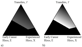
Figure 3. Multiplicative combination of the Metric (Figure 2a) and Boundary Condition (Figure 2b) Triangles (a). In (b), the gray scale is renormalized to highlight the minimum and maximum values.
2.5. Job Families with Low Numbers
While everything presented thus far has been shown as continuous plots, some of the groups being hired are in such small numbers that distinct points, as shown in Figure 4a and 4b, is more appropriate. (The plots are a discrete equivalent of the continuous plots in Figure 2.) While the analysis and how to determine the “Sweet Spot” is unchanged, the “Sweet Spot” itself moved from (18%, 61%, 21%) or (0.683, 0.183) to (36%, 18%, 46%) or (0.331, 0.400) owing to the situation where the discrete points, in this particular case, do not get as close to the cusp of the Boundary Condition plot as before, Figure 4c. However, the work done for Figure 2 can be done here and then adjusted to the closest low number point outside of the black excluded Boundary Condition areas. In this case, it is located at (14%, 63%, 23%) or (0.715, 0.200), which is slightly higher in Experienced and Transfers and slightly lower in Early Career hire than the full calculation. This point’s gray scale is only a few percent higher in gray scale than the “Hiring Sweet Spot” determined using only the low number calculation.
While the “Hiring Sweet Spot” might be just inside the excluded region of the Boundary Conditions, the decision to violate these conditions depends on their origin of that Boundary Condition. For example, a mentoring requirement can probably be adjusted slightly to allow an otherwise excluded “Hiring Sweet Spot”, but a Boundary Condition arising from a legal requirement probably does not have the same flexibility.
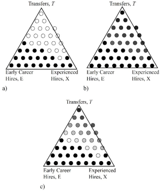
Figure 4. Graphical representation of a Metric (a, left) and a Boundary Condition (b, right) from Figure 2 with a low hire count. The combined triangle, Figure 4c, is the equivalent of Figure 3b. A black border was added to the circles in both plots in order to make the lighter circles clearer.
2.6. More Complex Boundary Conditions and Metrics
So far, the Metric examples are simple linear mathematical expressions and the gray scale changes uniformly across the triangle. In fact, no matter how many Metric Triangles with linear expressions are combined, the result will always have the expressions and the gray scale change uniformly across the triangle. Thus, no matter how many Metric Triangles with linear expressions are combined, the result will always have the maximum (and minimum by the way) at one of the vertices, along the entire length of one of the edges if two vertices are equally high, or no maximum if the triangle gray scale is uniform from edge-to-edge. (Although the word “maximum” is being used, some metrics, such as cost, are preferred with lower values. For those metrics, the gray scale is reversed so darker is less favorable and lighter is more favorable. Nevertheless, it will still be called “maximum” for consistency.)
However, Boundary Conditions are inherently non-linear, having a sharp shift between black and white. When they are combined with the Metrics, the minimum will be moved away from the vertices and, if the slope of a Boundary Condition is large enough and sufficiently complex so it is not a simple straight line, also away from the edges of the triangle. This is what happens in Figures 3 and 4 where the “Sweet Spot” is shifted away from each of the vertices and each of the edges in Figure 2.
That being said, more complex expressions can be used and are sometimes needed. These formulas can include dividing, multiplying, squaring, square root, and almost any other mathematical expressions. In developing mathematical formulas, since all the values are between 0 and 1, the usual expectation of increasing or decreasing a value is reversed. For example, squaring (or higher order exponentiation) values will cause resulting values to decrease (becoming a less favorable hiring space) while square root (or higher roots) of values will be larger (becoming a more favorable hiring space). If a particular function’s gray scale is backwards (low being desirable instead of high being desirable as shown in Figure 5), the actual metric can simply be subtracted from 1 or inverted (reciprocal) to reverse the gray scale.
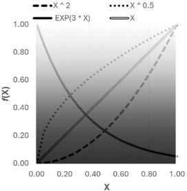
Figure 5. Examples of other mathematical functions that can be used for Metrics or Boundary Conditions.
2.7. A Multiplicative Metric Example (Synergy)
What about potential synergy between these three populations? Since we are looking at combinations of the populations, this would involve some combination of products of ε, χ, and τ along with other factors and constants. While the simplest such function is a product among the triplet values, ε * χ * τ, two scenarios are more interesting. The first still maintains the same exponent, n, in each of the factors, but has n >= 1.
SymmetricSynergy=εn χn τn133n(6)
As n increases, the width of the corresponding distribution decreases while, by symmetry, the peak clearly remains at (1/3, 1/3, 1/3). Synergy values along the vertical center line of the triangle are shown in Figure 6 for n = 1, 2, 4, and 10. (The other two components have identical plots along their respective axis through their vertices.)
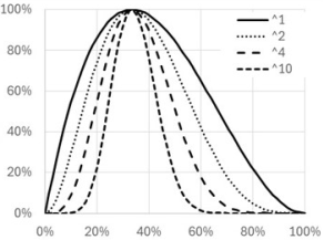
Figure 6. Plot of gray scale for Symmetric Synergy Formula, Equation (6), along the vertical axis (the Early Career-Experienced side of the triangle is 0% and the Transfers vertex is 100%.
The second scenario is when the exponents are not the same, for example.
AsymmetricSynergy=α εm χn τo13m+n+o(7)
Where α is a normalization factor so the values remain between 0 and 1. The normalization factor is not required in the Symmetric Synergy formula, Equation (6), since the maximum is always located at (0.500, 0.290) or (33.3%, 33.3%, 33.3%) and the denominator is the normalization factor. Figure 7 shows a symmetric plot where n = 2 (Figure 7a) and an asymmetric plot where m = 1, n = 2, and o = 3 (Figure 7b). In this case, b, the maximum is shifted away from Early Career and slightly to Experienced and strongly to Transfers. The actual coordinates are (0.582, 0.433) or (8%, 42%, 50%).
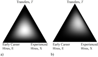
Figure 7. Plot of Symmetric Synergy with n = 2 (a, left) and Asymmetric Synergy with m = 1, n = 2, o = 3 (b, right).
2.8. More Complex Metrics
For a more practical (and complex) example, the total cost per unit of work (per week, per patient, or other units) over time can be calculated. While the cost is not the same as the employee’s salary, since this study is evaluating staffing, only the employee’s salary will be considered. However, we do need to account for the salaries and work for both an employee and their work mentor. (These numbers are very approximate and would need to be evaluated in each situation.)
If an Early Career nurse needs to be directly supervised 20% of the time by a more experienced nurse, nurse supervisor, or charge nurse, whose salary is 50% higher than the Early Career employees, the salary and number of hours would be
Salary = Early Career Salary×(100% + 20%×150%) = 130%×Early Career Salary(8)
Work Hours = 80%×Early Career
For the Experienced Nurse, much less oversight is needed, say 5% of the time (and also for a shorter period, but that is not considered here), but their salaries are closer to that of a senior nurse (for example, 140% of Early Career Nurses instead of the prior 150%). The total salary and number of hours for an Experienced nurse would then be
Salary = Early Career Salary x (140% + 5% x 150%) = 148% x Early Career Salary(9)
Work Hours = 95% x Early Career
So, the total cost per unit of work would be sum of Equations (8), (9), and the Transfer Employee’s Salary divided by the sum of Equations (8), (9), and the Transfer Employee’s Hours.
Initial Salary = 130% ε+148% χ+150% τ80% ε+95% χ+100% τ(10)
After 5 Years and assuming everyone get a 4% pay increase per year and the oversight requirement drops equally each year, the formula becomes
Salary at 5 Years = 122% ε+170% χ+182% τε+χ+τ(11)
and the “Hiring Sweet Spot” moves from Transfers to Early Career Hires, as shown in renormalized plots in Figure 8. (Although not shown, this transition occurs between years 2 and 3 with Experienced Hires becoming the “Hiring Sweet Spot” for part of that time. In addition, under these assumptions, the gap between the best and worst vertex increases each year.) Finally, the choice of 5 years and whether the time = 0, the time = 5, or the sum of each year 0 through year 5 is chosen for the cost/productivity metric is beyond the present scope of this publication.
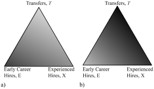
Figure 8. Annual Salaries per Unit Work at Time = 0 (a, left) and Time = 5 Years (b, right).
2.9. More Complex Boundary Conditions
Boundary Conditions are used as a binary True / False of including and excluding parts of the triplet space. Although the number of these conditions can be as many and they can be as complicated as required, two will be considered here, namely, having all types of staff and providing sufficient mentors for “New” staff. Since there are strengths (and weaknesses) of each type of new staff, it is desired to have a combination of these three staff types. In this example, each type of hire must be between 10% and 70% of the overall hires, Figure 9a.
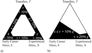
Figure 9. Examples of more complex Boundary Conditions of each value being between 10% and 70% inclusive (a) and requiring mentors by limiting t + 10% x >= e; t >= 20% x. The applicable Boundary Condition equations are shown in each section of (a) and (b).
The second situation is to make sure that each of the “new” staff members has sufficient mentoring or informal supervision by more experienced staff. To account for time off, different shifts, and other situations, the number of Early Career Hires will be forced to be less than the number of Transfers plus 10% of the number of Experienced Hires and that there are no more than 5 Experienced Hires for every Transfer. (These numbers are not necessarily the optimum for this situation. That would have to be determined for each specific situation.) This specific Boundary Condition plot is Figure 9b.
These two plots need to be combined using the previously discussed point-by-point multiplication of the gray scale. Afterwards, the possible hiring space is greatly reduced, Figure 10. So, Boundary Conditions, particularly the use of multiple Boundary Conditions, needs to be done cautiously.
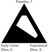
Figure 10. Combined Boundary Conditions from Figure 9 showing how quickly the possible hiring space can be reduced with seemingly reasonable conditions.
3. Results
3.1. Handling Multiple Metrics and Boundary Conditions
At this point, the discussion moves to a full example with multiple Boundary Conditions and Metrics. Table 3 shows a series of Metrics and Boundary Conditions. (They are far from being comprehensive.) Each of the characteristic groups have their respective advantages and disadvantages in terms of costs, productivity, and other metrics that have examined in various situations elsewhere and in many unpublished “White Papers”. In addition, these metrics and their importance vary from one job-family to another.
The results of these Metric and Boundary Condition Plots are in Figure 11. Since the number of Human Resources Business Partners being hired is much smaller than the number of Registered Nurses, low number plots similar to Figure 4 are used. In both of the combination plots the “Hiring Sweet Spot” is marked by concentric circles white and black circles. The “Hiring Sweet Spot” in the RN example (Figure 11 left) is (37%, 32%, 31%) and in the Human Resources Business Partner Example (Figure 11 right) is (6%, 48%, 46%).
Table 3. Examples of Characteristics and Boundary Conditions by Classifications.

Registered Nurse

Human Resources Business Partner

Weight

EC Hire

Exp. Hire

Xfer

Weight

EC Hire

Exp. Hire

Xfer

Metric

Experience

40%

ML

MH

MH

60%

L

MH

M

Cost

30%

ML

H

H

15%

M

MH

H

Productivity

20%

M

MH

H

5%

ML

MH

MH

Synergy (Equation (7))

10%

1

1

1

20%

1

2

2

Boundary Condition

Force All Types

EC: ≥ 10% and ≤ 50% Others: ≥ 10% and ≤ 80%

All: ≥ 10% and ≤ 50%

Mentor Needed

EC ≤ Xfer + 0.5 * Exp Exp. ≤ 4 * Xfer

NONE

Employee Type: EC — Early Career, Exp. — Experienced, Xfer – Transfer Metric Scale: Low (10%), Medium-Low (30%), Medium (50%), Medium-High (70%), High (90%)

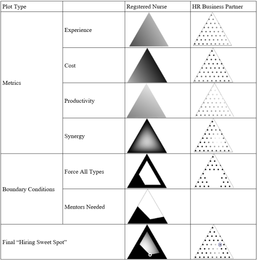
Figure 11. Full scale example using the Metrics and Boundary Conditions for a Registered Nurse and a Human Resources Business Partner as shown in Table 3. The “Hiring Sweet Spots” are shown as concentric black and white circles in the combination plots.
3.2. Adjusting the Hiring Target over Time
Just like Helmuth von Moltke the Elder’s famous quote that can be paraphrased that “No plan survives contact with the enemy” , no hiring plan survives the first hire. As the hiring continues, the current ratio of Early Career Hires, Experienced Hires, and Transfers will not be the optimum. (In addition, business conditions may change requiring a modification of the previous calculations, but that will not be considered here.) Consequently, a new target point that is a weighted reflection of the current ratio through the “Hiring Sweet Spot” can be determined. This becomes the target for future hiring that would be needed to bring the overall hiring for this facility in line with the previously determined “Hiring Sweet Spot”. For example, using the “Hiring Sweet Spot” of Figure 3, namely (18%, 61%, 21%), the “Hiring Sweet Spot” for hiring 100 employees gives a target of 18 Early Career Hires, 61 Experienced Hires, and 21 Transfers as shown as the “X” in Figure 12a. After 50 hires, suppose the actual hiring is 10 Early Career Hires, 20 Experienced Hires, and 20 Transfers (black circle in Figure 12b), the new target for future hiring would be 8 Early Career Hires, 41 Experienced Hires, and 1 Transfers in the remaining 50 hires or 16%, 82%, 2%, respectively, the square in Figure 12b, which is far from the original “Hiring Sweet Spot”.
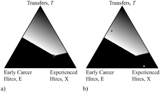
Figure 12. Over time, as the hiring process continues, the actual position in the hiring space shifts (from the “x” in a to the black circle in b). Consequently, a new target in the hiring space is needed (white square in b) so that the overall hiring remains at the calculated “Hiring Sweet Spot”.
If the current hiring situation is not re-evaluated frequently, it might become impossible to achieve the initial desired “Sweet Spot” hiring target. For example, in the above situation, if there had been 30 Early Career Hires in the initial 50 hires, it is not possible with the total projected number of employees to achieve the “Hiring Sweet Spot” as the number of Early Career Hires already exceeds the desired 18 Early Career Hires. This situation, assuming the other hires were 5 Transfers and 15 Experienced Hires, is shown in Figure 13 with the same symbols that were used in Figure 12 (although the colors are reversed). While achieving the original “Hiring Sweet Spot” is not possible since that hiring target (black square) is well outside of the triangle, a new hiring target (white star at (26%, 74%, 0%)) can be used to come as close as possible to original “Hiring Sweet Spot”. The new optimum (“x”) is located at (18%, 52%, 30%).
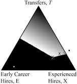
Figure 13. If the current position in the hiring space is not monitored and adjusted frequently enough, the current hiring position (white circle) might be so far from the “Hiring Sweet Spot” that a point outside the Triangle (black square) is needed to achieve the desired final hiring ratios. However, since this is not possible, a new future target (white star with a black border) can be determined to leave the final position in the hiring space (“x”) as close as possible to the initial “Hiring Sweet Spot”.
4. Discussion
In addition to determining the “Hiring Sweet Spot”, the same process can be used to determine the optimum ratio of certain jobs. One example is the ratio of Licensed Vocational Nurse (LVN) /Registered Nurse (RN) / Nurse Practitioner (NP) in a clinic or medical practice. (Including a Physician or Physicians in this analysis is very reasonable; however, as explained in the introduction, the resulting figure would be a 3-dimensional tetrahedron and is not easily illustrated on a 2-dimensional page, so Physicians were not added to this example.) While an NP can do everything that a LVN or an RN can do, they come with two major disadvantages, namely their cost not only in terms of salary but also in terms of office space and support staff and the overall population of NPs is much smaller than that of RNs because, in no small part, of the extensive additional training. Having a staff that is too heavy on the NP side would be inefficient, costly, and difficult to build or maintain. A staff that is too heavy in LVNs would leave the facility unable to meet the patient’s needs. The optimum situation is clearly a combination of the three roles based on some set of metrics and boundary conditions, which is exactly what was discussed here. This process will also show if there needs to optimum situation is what might otherwise be considered an imbalance, in order to achieve the expected facility’s patient load, procedure mix, and financial goals. Additional examples include the proportions of Dental Hygienist / Registered Dental Assistants / Dentists at a large dental practice. A two-characteristic example would be the ratio of Audiologists to Ear, Nose, and Throat (ENT) Doctors at an ENT practice with multiple physicians.
While the discussion so far has been based on a single health care facility, the process can be extended to any industry and organization location, comparing staffing at multiple locations, and even evaluating local versus overseas locations. Each of these different possibilities will need a different set of Metrics and Boundary Conditions that may have little relationship to those used in other situations. Each leadership team needs to determine what metrics and boundary conditions are important to their organization, business goals, and company philosophy.
5. Conclusions
Staffing a new facility of any type, but particularly a new medical facility is a daunting long-term task and hiring considerations should not be taken lightly (A paraphrase of the saying “Decide in haste; repent in leisure” is very appropriate in this situation.). A mathematical procedure to determine the optimum staffing based on a series of metrics and boundary conditions has been created and discussed. The choice of metrics and boundary conditions, relative weightings, and the respective value for each characteristic group depends on the particular industry, facility, and job-family mix. Examples of these metrics and boundary conditions in a three characteristic group situation, which can be easily visualized, were presented. The visualization is helpful, but not required, so the same process can be used for a larger group of characteristics without the visualizations. (Those visualizations would require the use of an application to view and rotate multi-dimensional figures).
Abbreviations

E or EC

Early Career Candidates

ENT

Ear Nose and Throat Physician

H

High Metric Value (90%)

HRBP

Human Resources Business Partner

L

Low Metric Value (10%)

LVN

Licensed Vocational Nurse

M

Medium Metric Value (50%)

MH

Medium-High Metric Value (70%)

ML

Medium-Low Metric Value (30%)

NP

Nurse Practitioner

RN

Registered Nurse

T or Xfer

Transferred Candidates

X or Exp

Experienced Candidates

Acknowledgments
The authors gratefully acknowledge discussions with L. A. Lieu and L. M Maldonado regarding the information in Table 3 of the Handling Multiple Metrics and Boundary Conditions section, which was, in turn, used to calculate and generate the images shown in Figure 11.
Author Contributions
R. B. Irwin: Conceptualization, Methodology, Software, Visualization, Writing – original draft, Writing – review & editing
C. E. Koch: Conceptualization, Methodology, Writing – review & editing
Data Availability Statement
All of the data used to generate the figures, with the exception of Figures 5 and 6, is given in the text, the figure captions, or the figures themselves. In Figures 5 and 6, the plots are derived from the formulas that are given in the text or in the figure. For the triangle “Sweet Spot” plots, the R Script used to generate the plots is given in the Appendix. That R script can be easily modified to generate any of those figures by modifying the rgb_shade functions. The provided R script is configured to generate the plots in Figures 2 and 3.
Conflicts of Interest
The authors declare no conflicts of interest.
Appendix
The following is an example of one of the R scripts that were used in calculating the results and generating these plots. The others can be developed from this one with minor modifications, primarily of the rgb_shade functions in lines 34—48 and 52—60 (line numbers are not shown but can be seen if the script is copied into RStudio or similar integrated development environment for R). The provided R script is configured to generate the plots in Figures 2 and 3.
#
# Heat Map Plot (Black/White Scale) of Boundary Condition Across an Equilateral Triangle Space
#
#
# This r Script is Adapted from https://stackoverflow.com/questions/76371621/gradient-fill-of-triangle-geom-polygon
#
#
# Check for Required Libraries and Install if Not Already Installed
#
if (!require(ggplot2)) install.packages('ggplot2')
if (!require(tidyverse)) install.packages('tidyverse')
if (!require(tidyverse)) install.packages('rstudioapi')
if (!require(dplyr)) install.packages('dplyr')
if (!require(purrr)) install.packages('purrr')
library(ggplot2)
library(tidyverse)
library(rstudioapi)
library ('dplyr')
library ('purrr')
#
# Set Variables
#
square_root_3 <- sqrt(3)
half_square_root_3 <- square_root_3 / 2
resolution <- 300 # About the Number of X-Axis Points
data_point_diameter <- 1
data_points_in_plot <- as.integer(resolution ^ 2 * square_root_3 / 2) # Provided as an FYI
current_script_path <- dirname(rstudioapi: : getSourceEditorContext()$path)
#
# Set the Black/White Color According to This Formula
# (Scale is 1 (White) to 0 (Black))
#
# Boundary Condition shade function
#
rgb_shade_bc <-function(x, y)
{
transfer <- abs(2 * square_root_3 * y / 3)
early <- abs((1 - x) - (square_root_3 * y / 3))
experienced <- abs(x - square_root_3 * y / 3)
if((transfer >= early)
& (transfer >= experienced / 3)
)
{
return(1)
}else{
return(0)
}
}
#
# Metric shade function
#
rgb_shade_metric <-function(x, y)
{
transfer_value <- 0.90
early_career_value <- 0.20
experienced_value <- 0.40
color_change_x <- experienced_value - early_career_value
color_change_y <-(transfer_value - early_career_value - 0.5 * color_change_x) / half_square_root_3
return(median(c(0, early_career_value + color_change_y * y + color_change_x * x, 1)))
}
#
# Set Up Points of Triangle
# Triangle Height is the Resolution * 3^0.5 / 2
# X Limits are (Y / 3^0.5) to 1 - (Y / 3^0.5)
#
# ": " Gives Integer Values Between the Given Limits; Multiplying by "Resolution" Gives "Resolution" Number of Points
# Subsequently Dividing by "Resolution" Gives Values Between 0 and 1 for x and y
#
# The Median Function Corrects for Any Colors Being Outside of [0, 1]
#
triangle_bc <- map((1: (resolution * square_root_3 / 2)) / resolution, \(y)
{
map(((y * resolution / square_root_3): (resolution - y * resolution / square_root_3)) / resolution, \(x)
{
tibble(
x = x,
y = y,
shade = rgb_shade_bc(x, y),
color = rgb(shade, shade, shade)
)
})
}) |> list_flatten() |> list_rbind()
triangle_metric <- map((1: (resolution * square_root_3 / 2)) / resolution, \(y)
{
map(((y * resolution / square_root_3): (resolution - y * resolution / square_root_3)) / resolution, \(x)
{
tibble(
x = x,
y = y,
shade = rgb_shade_metric(x, y),
color = rgb(shade, shade, shade))
})
}) |> list_flatten() |> list_rbind()
triangle_combined <- map((1: (resolution * square_root_3 / 2)) / resolution, \(y)
{
map(((y * resolution / square_root_3): (resolution - y * resolution / square_root_3)) / resolution, \(x)
{
tibble(
x = x,
y = y,
color = rgb(median(c(0, rgb_shade_metric(x, y) * rgb_shade_bc(x, y), 1)),
median(c(0, rgb_shade_metric(x, y) * rgb_shade_bc(x, y), 1)),
median(c(0, rgb_shade_metric(x, y) * rgb_shade_bc(x, y), 1))),
shade = rgb_shade_metric(x, y) * rgb_shade_bc(x, y)
)
})
}) |> list_flatten() |> list_rbind()
#
# Find the Maximum Value Location
#
sweet_spot_x <- triangle_combined$x [which.max(triangle_combined$shade)]
sweet_spot_y <- triangle_combined$y [which.max(triangle_combined$shade)]
sweet_spot_color <- triangle_combined$color [which.max(triangle_combined$shade)]
sweet_spot_shade <- triangle_combined$shade [which.max(triangle_combined$shade)]
sweet_spot_transfers <- sweet_spot_y * 2 / square_root_3
sweet_spot_experienced <- sweet_spot_x - sweet_spot_transfers / 3
sweet_spot_early_career <- 1.0 - sweet_spot_experienced - sweet_spot_transfers
#
# Re-Normalize the Metric Triangle
#
triangle_normalized <- map((1: (resolution * square_root_3 / 2)) / resolution, \(y)
{
map(((y * resolution / square_root_3): (resolution - y * resolution / square_root_3)) / resolution, \(x)
{
tibble(
x = x,
y = y,
color = rgb(median(c(0, rgb_shade_metric(x, y) * rgb_shade_bc(x, y) / sweet_spot_shade, 1)),
median(c(0, rgb_shade_metric(x, y) * rgb_shade_bc(x, y) / sweet_spot_shade, 1)),
median(c(0, rgb_shade_metric(x, y) * rgb_shade_bc(x, y) / sweet_spot_shade, 1))),
shade = rgb_shade_metric(x, y) * rgb_shade_bc(x, y)
)
})
}) |> list_flatten() |> list_rbind()
#
# Move the Plot Up Slightly for the "Early Career Hires" and the "Experienced Hires"
#
triangle_bc [, 'y'] <- triangle_bc [, 'y'] + 0.02
triangle_metric [, 'y'] <- triangle_metric [, 'y'] + 0.02
triangle_combined [, 'y'] <- triangle_combined [, 'y'] + 0.02
triangle_normalized [, 'y'] <- triangle_normalized [, 'y'] + 0.02
#
# Plot the Triangles
#
triangle_bc |> ggplot(aes(x, y, colour = color)) +
geom_point(size=data_point_diameter) +
scale_colour_identity() +
coord_equal() +
theme_void() +
annotate("text", x = 0.5, y = 0.91, label = "Transfers", colour = "black") +
annotate("text", x = 0.1, y = 0, label = "Early Career Hires", colour = "black") +
annotate("text", x =.9, y = 0, label = "Experienced Hires", colour = "black")
triangle_metric |> ggplot(aes(x, y, colour = color)) +
geom_point(size=data_point_diameter) +
scale_colour_identity() +
coord_equal() +
theme_void() +
annotate("text", x = 0.5, y = 0.91, label = "Transfers", colour = "black") +
annotate("text", x = 0.1, y = 0, label = "Early Career Hires", colour = "black") +
annotate("text", x =.9, y = 0, label = "Experienced Hires", colour = "black")
triangle_combined |> ggplot(aes(x, y, colour = color)) +
geom_point(size=data_point_diameter) +
scale_colour_identity() +
coord_equal() +
theme_void() +
annotate("text", x = 0.5, y = 0.91, label = "Transfers", colour = "black") +
annotate("text", x = 0.1, y = 0, label = "Early Career Hires", colour = "black") +
annotate("text", x =.9, y = 0, label = "Experienced Hires", colour = "black")
triangle_normalized |> ggplot(aes(x, y, colour = color)) +
geom_point(size=data_point_diameter) +
scale_colour_identity() +
coord_equal() +
theme_void() +
annotate("text", x = 0.5, y = 0.91, label = "Transfers", colour = "black") +
annotate("text", x = 0.1, y = 0, label = "Early Career Hires", colour = "black") +
annotate("text", x =.9, y = 0, label = "Experienced Hires", colour = "black")
#
# Save as.csv to Same Folder as the R Script
#
write.csv(triangle_bc,
paste(dirname(rstudioapi: : getSourceEditorContext()$path),
'/',
'Figure_2a_Boundary_Condition',
'.csv',
sep = ''),
row.names = FALSE)
write.csv(triangle_metric,
paste(dirname(rstudioapi: : getSourceEditorContext()$path),
'/',
'Figure_2b_Metric',
'.csv',
sep = ''),
row.names = FALSE)
write.csv(triangle_combined,
paste(dirname(rstudioapi: : getSourceEditorContext()$path),
'/',
'Figure_3_Combined',
'.csv',
sep = ''),
row.names = FALSE)
write.csv(triangle_normalized,
paste(dirname(rstudioapi: : getSourceEditorContext()$path),
'/',
'Figure_4_Renormalized',
'.csv',
sep = ''),
row.names = FALSE)
References
[1] Dussault, G., Dubois, C. A.: Human resources for health policies: a critical component in health policies. Human Resources for Health 1, 1 (2003).
[2] Kabene, S. M., Orchard, C., Howard, J. M. et al.: The importance of human resources management in health care: a global context. Human Resources for Health 4, 20 (2006).
[3] Gile, P. P., Buljac-Samardzic, M. & Klundert, J. V.: The effect of human resource management on performance in hospitals in Sub-Saharan Africa: a systematic literature review. Human Resources for Health 16, 34 (2018).
[4] Mitchell, C. C., Ashley, S. W., Zinner, M. J., & Moore, F. D. Predicting future staffing needs at teaching hospitals: use of an analytical program with multiple variables. Archives of Surgery, 142(4), 329-334 (2007).
[5] Humphries, N., Morgan, K., Catherine Conry, et al.: Quality of care and health professional burnout: narrative literature review. International Journal of Health Care Quality Assurance, 27(4), 293-307 (2014).
[6] Kane, R. L., Shamliyan, T. A., Mueller, C., et al.: The association of registered nurse staffing levels and patient outcomes: systematic review and meta-analysis. Medical Care. 45(12): 1195–204 (2007).
[7] Dall’Ora C., Saville C., Rubbo B., et al.: Nurse staffing levels and patient outcomes: a systematic review of longitudinal studies. International Journal of Nursing Studies, 134: 104311 (2022).
[8] Gerdtz, M. F., Nelson, S.: 5-20: a model of minimum nurse-to-patient ratios in Victoria, Australia. Journal of Nursing Management 15(1): 64–71 (2007).
[9] Van den Heede, K., Cornelis, J., Bouckaert, N., et al.: Safe nurse staffing policies for hospitals in England, Ireland, California, Victoria and Queensland: a discussion paper. Health Policy. 124(10): 1064–73 (2020).
[10] McHugh, M. D., Aiken, L. H., Needleman, S. J., et al.: Nurse Staffing and Inpatient Hospital Mortality, New England Journal of Medicine 364(11), 1037-1045 (2011).
[11] Aiken, L. H., Clarke, S. P., Sloane, D. M., et al.: Hospital Nurse Staffing and Patient Mortality, Nurse Burnout, and Job Dissatisfaction. Journal of the American Medical Association. 288(16): 1987–1993 (2002).
[12] Aiken, L. H., Clarke, S. P., Sloane, D. M.: Hospital staffing, organization, and quality of care: cross-national findings, International Journal for Quality in Health Care, 14 (1), 5–14 (2002).
[13] Unruh, L.: Nurse staffing and patient, nurse, and financial outcomes. The American Journal of Nursing, 108(1), 62-71 (2008).
[14] Morioka, N., Okubo, S., Moriwaki, M., & Hayashida, K.: Evidence of the association between nurse staffing levels and patient and nurses’ outcomes in acute care hospitals across Japan: a scoping review. Healthcare 10(6), 1052 (2002).
[15] Park, S. H., Blegen, M. A., Spetz, J., et al.: Comparison of nurse staffing measurements in staffing-outcomes research. Medical Care, 53(1), e1-e8 (2015).
[16] Dall’Ora, C., Rubbo, B., Saville, C. et al.: The association between multi-disciplinary staffing levels and mortality in acute hospitals: a systematic review. Human Resources for Health 21, 30 (2023).
[17] Cartmill, L., Comans, T. A., Clark, M. J. et al.: Using staffing ratios for workforce planning: evidence on nine allied health professions. Human Resources for Health 10, 2 (2012).
[18] Asamani, J. A., Amertil, N. P., & Chebere, M.: The influence of workload levels on performance in a rural hospital. British Journal of Healthcare Management, 21(12), 577-586 (2015).
[19] Schoo, A. M., Boyce, R. A., Ridoutt, L. S. T.: Workload capacity measures for estimating allied health staffing requirements. Australian Health Review 32, 548-558 (2008).
[20] Flynn, M., McKeown, M.: Nurse staffing levels revisited: a consideration of key issues in nurse staffing levels and skill mix research. Journal of Nursing Management, 17(6), 759-766 (2009).
[21] Johannsen, S. A., Roberts, D. A., Smith, L. A., et al, Pastoral Care Department Staffing Algorithm Pilot Project [Poster Presentation], Association of Professional Chaplains (APC) / National Association of Catholic Chaplains (NACC) Joint Conference, St. Louis, Missouri, USA, June 20-23, 2024.
[22] Nagy, B., Abuhmaidan, K.: A Continuous Coordinate System for the Plane by Triangular Symmetry, Symmetry 11(2) 191 (2019).
[23] Braden, B.: The Surveyor's Area Formula (PDF). The College Mathematics Journal. 17(4): 326–337 (1986).
[24] Ballantine, J. P., Jerbert, A. R.: Distance from a Line, or Plane, to a Point. The American Mathematical Monthly, 59(4), 242–243 (1952).
[25] R Core Team: R: A Language and Environment for Statistical Computing. R Foundation for Statistical Computing, Vienna, Austria (2023).
[26] Lappi, E.: New hires, adjustment costs, and knowledge transfer—evidence from the mobility of entrepreneurs and skills on firm productivity, Industrial and Corporate Change, Volume 33, Issue 3, Pages 712–737 (2024).
[27] Blatter, M., Muehlemann, S., Schenker, S.: The costs of hiring skilled workers, European Economic Review, 56(1), 20-35, (2012).
[28] Papay, J. P., Kraft, M. A.: The Productivity Costs of Inefficient Hiring Practices: Evidence from Late Teacher Hiring. Journal of Policy Analysis and Management 35(4): 791-817 (2016).
[29] Muehlemann, S., Leiser, M. S.: Hiring costs and labor market tightness, Labour Economics, 52, 122-131 (2018).
[30] Moltkes Militärische Werke: II. Die Thätigkeit als Chef des Generalstabes der Armee im Frieden. (Moltke’s Military Works: II. Activity as Chief of the Army General Staff in Peacetime) Zweiter Theil (Second Part), Aufsatz vom Jahre 1871 Ueber Strategie (Article from 1871 on strategy), Start Page 287, Quote Page 291, Publisher: Ernst Siegfried Mittler und Sohn, Berlin, Germany, 1900. A similar quote has been attributed to Sun Szu in “The Art of War” (5th Century BC), Napolean Bonaparte (early 1800s), and Carl von Clausewitz (circa 1820s).
[31] Congreve, W: Comedy of manners titled “The Old Batchelour” (1693). A paraphrase of the adage on marriage, “Married in haste, we may repent at leisure.”
[32] RStudio Team: RStudio: Integrated Development for R. RStudio, PBC, Boston, MA (2020).
Cite This Article
  • APA Style

    Irwin, R. B., Koch, C. E. (2026). Optimizing Staffing for a New Medical Facility. Journal of Human Resource Management, 14(2), 144-157. https://doi.org/10.11648/j.jhrm.20261402.15

    Copy | Download

    ACS Style

    Irwin, R. B.; Koch, C. E. Optimizing Staffing for a New Medical Facility. J. Hum. Resour. Manag. 2026, 14(2), 144-157. doi: 10.11648/j.jhrm.20261402.15

    Copy | Download

    AMA Style

    Irwin RB, Koch CE. Optimizing Staffing for a New Medical Facility. J Hum Resour Manag. 2026;14(2):144-157. doi: 10.11648/j.jhrm.20261402.15

    Copy | Download

  • @article{10.11648/j.jhrm.20261402.15,
      author = {R. B. Irwin and C. E. Koch},
      title = {Optimizing Staffing for a New Medical Facility},
      journal = {Journal of Human Resource Management},
      volume = {14},
      number = {2},
      pages = {144-157},
      doi = {10.11648/j.jhrm.20261402.15},
      url = {https://doi.org/10.11648/j.jhrm.20261402.15},
      eprint = {https://article.sciencepublishinggroup.com/pdf/10.11648.j.jhrm.20261402.15},
      abstract = {When a new medical facility is planned, there is a need for staff members of various job roles and levels. For each of these roles, there are several different classifications for staff. Each of these classification groups have their respective advantages and disadvantages in terms of cost, productivity, new ideas, and other characteristics. Some of these characteristics have a continuous range of values, which differ for each type of job role. In addition, there are boundary conditions characteristics, which only have binary values (True/False), that also limit the proportion for each classification group. While the number of classifications is not limited, this publication will consider examples with three primary classifications for staff: early career hires, experienced hires, and (experienced) transfers. This article details a method for using these metrics and boundary conditions to optimize the staffing using a visualization approach. While the equations for the metrics and boundary conditions can be solved directly and we show how that can be done, they do not answer how the optimum solution is obtained in the way that visualizations can. Since each facility and location may have its own unique requirements, this article discusses general principles and mathematical processes rather than exact prescriptions.},
     year = {2026}
    }
    

    Copy | Download

  • TY  - JOUR
    T1  - Optimizing Staffing for a New Medical Facility
    AU  - R. B. Irwin
    AU  - C. E. Koch
    Y1  - 2026/04/16
    PY  - 2026
    N1  - https://doi.org/10.11648/j.jhrm.20261402.15
    DO  - 10.11648/j.jhrm.20261402.15
    T2  - Journal of Human Resource Management
    JF  - Journal of Human Resource Management
    JO  - Journal of Human Resource Management
    SP  - 144
    EP  - 157
    PB  - Science Publishing Group
    SN  - 2331-0715
    UR  - https://doi.org/10.11648/j.jhrm.20261402.15
    AB  - When a new medical facility is planned, there is a need for staff members of various job roles and levels. For each of these roles, there are several different classifications for staff. Each of these classification groups have their respective advantages and disadvantages in terms of cost, productivity, new ideas, and other characteristics. Some of these characteristics have a continuous range of values, which differ for each type of job role. In addition, there are boundary conditions characteristics, which only have binary values (True/False), that also limit the proportion for each classification group. While the number of classifications is not limited, this publication will consider examples with three primary classifications for staff: early career hires, experienced hires, and (experienced) transfers. This article details a method for using these metrics and boundary conditions to optimize the staffing using a visualization approach. While the equations for the metrics and boundary conditions can be solved directly and we show how that can be done, they do not answer how the optimum solution is obtained in the way that visualizations can. Since each facility and location may have its own unique requirements, this article discusses general principles and mathematical processes rather than exact prescriptions.
    VL  - 14
    IS  - 2
    ER  - 

    Copy | Download

Author Information
  • Health Catalyst, South Jordan, United States

  • Baylor Scott & White Health, Temple, United States

  • Abstract
  • Keywords
  • Document Sections

    1. 1. Introduction
    2. 2. Materials and Methods
    3. 3. Results
    4. 4. Discussion
    5. 5. Conclusions
    Show Full Outline
  • Abbreviations
  • Acknowledgments
  • Author Contributions
  • Data Availability Statement
  • Conflicts of Interest
  • Appendix
  • References
  • Cite This Article
  • Author Information