On the Performance of Some Estimation Methods in Models with Heteroscedasticity and Autocorrelated Disturbances (A Monte-Carlo Approach)

Olufemi Aderemi Ayansola; Adebowale Olusola Adejumo

doi:doi:10.11648/j.mma.20240901.13

Research Article |

| Peer-Reviewed

On the Performance of Some Estimation Methods in Models with Heteroscedasticity and Autocorrelated Disturbances (A Monte-Carlo Approach)

Olufemi Aderemi Ayansola^*, Adebowale Olusola Adejumo

Published in Mathematical Modelling and Applications (Volume 9, Issue 1)

Received: 3 December 2023 Accepted: 25 December 2023 Published: 2 April 2024

Views: Downloads:

Download PDF

Share This Article

Twitter
Linked In
Facebook

Abstract

The proliferation of panel data studies has been greatly motivated by the availability of data and capacity for modelling the complexity of human behaviour than a single cross-section or time series data and these led to the rise of challenging methodologies for estimating the data set. It is pertinent that, in practice, panel data are bound to exhibit autocorrelation or heteroscedasticity or both. In view of the fact that the presence of heteroscedasticity and autocorrelated errors in panel data models biases the standard errors and leads to less efficient results. This study deemed it fit to search for estimator that can handle the presence of these twin problems when they co- exists in panel data. Therefore, robust inference in the presence of these problems needs to be simultaneously addressed. The Monte-Carlo simulation method was designed to investigate the finite sample properties of five estimation methods: Between Estimator (BE), Feasible Generalized Least Square (FGLS), Maximum Estimator (ME) and Modified Maximum Estimator (MME), including a new Proposed Estimator (PE) in the simulated data infected with heteroscedasticity and autocorrelated errors. The results of the root mean square error and absolute bias criteria, revealed that Proposed Estimator in the presence of these problems is asymptotically more efficient and consistent than other estimators in the class of the estimators in the study. This is experienced in all combinatorial level of autocorrelated errors in remainder error and fixed heteroscedastic individual effects. For this reason, PE has better performance among other estimators.

Published in	Mathematical Modelling and Applications (Volume 9, Issue 1)
DOI	10.11648/j.mma.20240901.13
Page(s)	23-31
Creative Commons	This is an Open Access article, distributed under the terms of the Creative Commons Attribution 4.0 International License (http://creativecommons.org/licenses/by/4.0/), which permits unrestricted use, distribution and reproduction in any medium or format, provided the original work is properly cited.
Copyright	Copyright © The Author(s), 2024. Published by Science Publishing Group

Keywords

Modified, Method, Panel, Estimator, Simulations

1. Introduction

Panel data model have become increasingly popular in the past decades with the increased availability of cross country data sets.

[15]

, were the first set of scholars to work on panel data. Panel data describes the number of individuals across a sequence of time periods. There are several key advantages of using panel data over a single time series or cross-section data set. This combination of time series with cross-section can enhance the quality and quantity of data in ways that would be possible using only one of these two dimensions. To realize the potential value of the information contained in a panel data, see

[3, 4, 6, 9, 11, 27, 28]

Panel data typically contains some form of heteroscedasticity, serial correlation and /or spatial correlation. Therefore, robust inference in the presence of heteroscedasticity and serial correlation is an important problem in spatial data analysis,

[14]

The essence of these two problems is that, in many econometrics studies, including panel study, the assumption of constant variance for the disturbance term is unrealistic. This, then calls for a restrictive assumptions for panel, where, in practice, the cross-sectional units may be of varying size and as a result exhibit different variation.

It was observed that some scholars, consider cases where one accounts for heteroscedasticity and ignores the possibility of serial correlation problems in the model and vice-versa

[10]	Holly, A., Gardiol, I (2000). A Score test for Individual Heteroscedasticity in a One-Way Error Components Model.
[12]	Jaba, E., Robu, I. B., Istrate, C., Balan, C. B., Roman, M. (2016). The Statistical Assessment of the Value Relevance of Financial Information Reported by Romanian Listed Companies, Romanian Journal of Economic Forecasting, 19(2), pp. 27-42.
[13]	Jirata M. T, Chelule J. C. and Odhiambo R. O (2014) Deriving Some Estimators of Panel Data Regression Models With Individual Effects, International Journal of Science and Research, Volume 3 Issue 5.
[16]	Li, Q. and T. Stengos (1994). Adaptive Estimation in the Panel Data Error Component Model with Heteroscedasticity of Unknown Form, International Economic Review, 35: 981-1000.
[17]	Mazodier, P. and A. Trognon,(1978), Heteroskedasticity and Stratification in Error Component Models. Annales de VINSEE 30-31. 451-482.
[18]	Magnus, J. R. (1982). Multivariate Error Components Analysis of Linear and Non-linear Regression models by Maximum Likelihood, Journal of Econometrics 19, 239-285.
[19]	Olajide J. T. and Olubusoye, O. E. (2014) Estimating Dynamic Panel Data Models with Random Individual Effect: Instrumental Variable and GMM Approach.
[20]	Olajide, J. T, Ayansola O. A and Oyenuga, I. F (2017). Estimation of Dynamic panel Data Models with Autocorrelated disturbance term: GMM approach. Paper presented at 1^st international conference of Nigeria Statistical Society on Statistical Research and its Applications.
[22]	Phemelo (2018). Dynamic Panel Data Analysis of the Impact of Public Sector Investment on Private Sector Investment Growth in Sub-Saharan African.
[23]	Roy, N. (2002). Is Adaptive Estimation Useful for Panel Models with Heteroscedasticity in the Individual Specific Error Component? Some Monte Carlo Evidence, Econometric Reviews, 21: 189-203.
[24]	Randolph, W. C., (1998). A Transformation for Heteroscedastic Error Components Regression Models, Economics Letters 27: 349-354.
[25]	Uthman and Oyenuga (2021). A Monte- Carlo study of Dynamic Panel Data Estimators with Autocorrelated Error Terms. International Journal of Research/P-ISSN: 2348-6848, Volume 08 Issue 02.
[26]	Wansbeek, T. J. (1989). An Alternative Heteroscedastic Error Component Model, Econometric Theory 5, 326.

[10, 12, 13, 16, 17-20, 22-26]

. Few authors that consider both problems include

[1-3, 7, 8, 21]

. Of these authors, Baltagi et al, as well as both derived test for joint occurrence of heteroscedasticity and autocorrelation in one way and two-way error components respectively

[3, 21]

. The difference between this work and that of

[3]

is that it focuses on the development of a new estimator and estimation of the parameters not testing for the presence of autocorrelation and heteroscedasticity in the context of a panel data regression model.

Furthermore, this study explicitly decomposes error term as the sum of two elements; capturing individual heterogeneity and autocorrelation in the remainder error term. By so doing, the data is then generated from the error component model with serial correlation and heteroscedasticity with the help of Monte-Carlo Simulation method.

The study was mainly targeted at investigating finite sample properties of five estimation methods of panel data models in the presence of autocorrelation and heteroscedasticity in one-way error component model. The estimation methods are BE, FGLS, M, MM and PE.

The inclusion of M and MM estimators in this study is due to their performance in the various work

[29]

2. Methodology

2.1. Model Specification

Consider the following panel data model:

y_{it} = X_{it}^{1} β + u_{it,} i = 1, \dots, N; t = 1, \dots, T .

(1)

where: β is K × 1 vector of regression coefficient.

y_{it}

represent the response variable;

x_{it}

represent the regressors;

u_{it}

represent disturbance term

The disturbance follow one-way error component model

u_{it} = μ_{i} + v_{it}

(2)

μ_{i} ~ IID (0, σ_{μi}^{2})

and

v_{it}

follows AR(1) i.e.

v_{it} = {ρv}_{i, t - 1} + ε_{it}

(3)

Where

2.2. Monte-Carlo Experiment

This work present a Monte-Carlo experiment that studied the finite sample properties of the five estimation methods; Between estimator (BE), Feasible Generalized Least Square (FGLS), Maximum estimator (M), Modified Maximum estimator (MM) and Proposed estimator (PE) applied to panel data model.

The Root Mean Square Error (RMSE) were used as criterion to assess the performances of these estimators.

The set- up in the experiment in this study was based on both individual- specific effect and remainder disturbance simultaneously with joint assumptions of heteroscedasticity and AR(1); generating contaminated data.

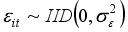
2.3. Data Generating Scheme

The design of Monte- Carlo experiments in this study uses the following information to generate infected data.

Consider the following panel model:

(4)

where

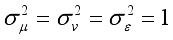
The parameters were assigned as.

The cross- sections and time periods was chosen as N= 25,100,200 and T= 5, 10. For each combinations of N and T; 5000 replications were considered.

The autocorrelation coefficient values and heteroscedasticity used are specified as

ρ

varies as 0.3, 0.5, 0.8 and

σ_{μ}^{2} (1 + λ {\overset{̅}{x}}_{i})

λ = 1 .

The variance of individual effects, remainder error and error term is one. i.e.

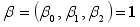
2.4. Derivation of a New Proposed Panel Data Estimator

Consider the likelihood function of the normal distribution as follows;

\frac{1}{({2 π)}^{\frac{n}{2}} {| V |}^{1 / 2}} e^{\frac{- 1}{2} U^{`} V^{- 1} U}

(5)

where

U = Y - Xβ

Therefore

L =

\frac{1}{({2 π)}^{\frac{n}{2}} {| V |}^{1 / 2}} e^{\frac{- 1}{2} (Y - Xβ) ` V^{- 1} (Y - Xβ)}

(6)

Assume that there exist, linear restriction

binding the regression coefficients vector of

, where R is a row vector of ones defined as

\frac{1}{K} (1, 1 \dots 1)

(6) is transformed, subject to constraint Rβ, as follows:

l = {(2 π)}^{\frac{- n}{2}} {|v|}^{- \frac{1}{2}} e^{\frac{- 1}{2} (Y - Xβ) ` V^{- 1} (Y - Xβ) - Rβ}

(7)

Taking natural logarithm of (7), we have,

\log_{e} l = - \frac{n}{2} \log_{e} (2 π) - \frac{1}{2} \log_{e} |V| - \frac{1}{2} {(Y - Xβ)}^{1} V^{- 1} (Y - Xβ) - Rβ

.(8)

\log_{e} l = - \frac{n}{2} \log_{e} (2 π) - \frac{1}{2} \log_{e} |V| - \frac{1}{2} [Y^{1} V^{- 1} Y

Y^{1} V^{- 1} Xβ - β^{1} X^{1} V^{- 1} Y + β^{1} X^{1} V^{- 1} X β] - Rβ

\log_{e} l = - \frac{n}{2} \log_{e} (2 π) - \frac{1}{2} \log_{e} |V| - \frac{1}{2} [Y^{1} V^{- 1} Y

2 X^{1} V^{- 1} Yβ + β^{1} X^{1} V^{- 1} Xβ] - Rβ

\log_{e} l = - \frac{n}{2} \log_{e} (2 π) - \frac{1}{2} \log_{e} |V| - \frac{1}{2} [Y^{1} V^{- 1} Y

2 X^{1} V^{- 1} Yβ + β^{1} X^{1} V^{- 1} Xβ + 2 Rβ]

By maximizing the log- likelihood function, therefore,

Let

\log_{e} l = A

\frac{\partial A}{\partial β} = - \frac{1}{2} [- 2 X^{1} V^{- 1} Y + 2 (X^{1} V^{- 1} X) β + 2 R]

\frac{\partial A}{\partial β} = X^{1} V^{- 1} Y - (X^{1} V^{- 1} X) β - R

Setting

\frac{\partial A}{\partial β} = 0

It implies that:

{0 = X}^{1} V^{- 1} Y - (X^{1} V^{- 1} X) β - R

Therefore,

{(X^{1} V^{- 1} X) β = X}^{1} V^{- 1} Y - R

Pre-multiply by

{(X^{1} V^{- 1} X)}^{- 1}

, it results into:

β_{P} {{= (X}^{1} V^{- 1} X)}^{- 1} X^{1} V^{- 1} Y - R {{(X}^{1} V^{- 1} X)}^{- 1}

(9)

Var

(β_{p}) = E [(β_{P} - β) {(β_{P} - β)}^{1}]

From (9),

β_{P} {{= (X}^{1} V^{- 1} X)}^{- 1} X^{1} V^{- 1} (Xβ + U) - R {{(X}^{1} V^{- 1} X)}^{- 1}

(10)

β_{P} {{= (X}^{1} V^{- 1} X)}^{- 1} X^{1} V^{- 1}

β + {{(X}^{1} V^{- 1} X)}^{- 1} X^{1} V^{- 1} U - R {{(X}^{1} V^{- 1} X)}^{- 1}

β_{P} = β + {{(X}^{1} V^{- 1} X)}^{- 1} X^{1} V^{- 1} U - R {{(X}^{1} V^{- 1} X)}^{- 1}

(11)

β_{P} - β = {{(X}^{1} V^{- 1} X)}^{- 1} X^{1} V^{- 1} U - R {{(X}^{1} V^{- 1} X)}^{- 1}

(12)

Therefore,

Var(

β_{P}

)=E[

{{(X}^{1} V^{- 1} X)}^{- 1} X^{1} V^{- 1} U - R {{(X}^{1} V^{- 1} X)}^{- 1}] {{{[(X}^{1} V^{- 1} X)}^{- 1} X^{1} V^{- 1} U - R {{(X}^{1} V^{- 1} X)}^{- 1}]}^{1}

Var(

β_{P}

{{(X}^{1} V^{- 1} X)}^{- 1} X^{1} V^{- 1} E (U U^{1}) X {{(X}^{1} V^{- 1} X)}^{- 1} + R {{(X}^{1} V^{- 1} X)}^{- 1} {{(X}^{1} V^{- 1} X)}^{- 1} R^{1}

Var(

β_{P}

σ^{2} {{(X}^{1} V^{- 1} X)}^{- 1} + R {{(X}^{1} V^{- 1} X)}^{- 1} {{(X}^{1} V^{- 1} X)}^{- 1} R^{1}

(13)

Bias ⌊\hat{β}⌋ = E ⌊\hat{β}⌋ - β = E ⌊\hat{β} - β⌋

(14)

E (β_{P} - β) = E [{{(X}^{1} V^{- 1} X)}^{- 1} X^{1} V^{- 1} U - R {{(X}^{1} V^{- 1} X)}^{- 1}]

E (β_{P} - β) = [{{(X}^{1} V^{- 1} X)}^{- 1} X^{1} V^{- 1} E (U) - R {{(X}^{1} V^{- 1} X)}^{- 1}]

Recall:

E (U) = 0

E (β_{P} - β) = - R {{(X}^{1} V^{- 1} X)}^{- 1}

(15)

ABias(

β

)

= |E (β_{P} - β)| = R {{(X}^{1} V^{- 1} X)}^{- 1} .

(16)

3. Results

In this analysis, attention is focused on the asymptotic behaviour of five estimators in panel data infected with autocorrelated error terms of low, moderate and high levels and heteroscedastic structure. Monte-Carlo experiment is used to generate infectious data. 5000 replications are performed on combination of cross section, N=25,100 and 200 and time periods, T=5 and 10 for different degrees of autocorrelation and heteroscedastic structure (0.3, 0.5, and 0.8). R- Package is used for the analysis.

Table 1. Root Mean Square Error in the Presence of Heteroscedasticity and Low Autocorrelation.

N			T=5			T=10
N		β₀	β₁	β₂	β₀	β₁	β₂
25	BE	0.00436	0.13246	0.11342	0.17371	0.03544	0.22084
	FGLS	0.04683	0.22915	0.61354	0.11077	0.77631	0.01124
	ME	0.00437	0.13246	0.11343	0.17371	0.03544	0.22084
	MME	0.06349	0.0681	0.24825	0.0499	0.03942	0.22238
	PE	0.00021	0.00031	0.00078	0.00399	0.00011	0.00356
100	BE	3.72E-06	3.82E-08	0.03066	0.00037	0.00011	0.01132
	FGLS	0.00075	0.00662	0.04158	0.0002	0.00785	0.05017
	ME	3.70E-06	0.00394	0.03066	0.00037	0.00011	0.01132
Ugkl;	MME	0.01193	0.00961	0.05442	0.00866	0.00712	0.03283
	PE	5.29E-06	0.00019	0.00047	0.000017	1.02E-04	0.00039
200	BE	0.00018	5.37E-05	0.00566	0.00031	0.00244	0.00098
	FGLS	0.0001	0.00393	0.02509	0.00422	0.01802	0.00233
	ME	0.00018	5.37E-05	0.00566	0.00031	0.00244	0.00098
	MME	0.00569	0.00457	0.02635	0.00604	0.00592	0.02736
	PE	0.000002	6.1E-07	0.00019	5.15E-06	0.000042	0.000027

Proposed estimator outperforms other estimators.

Table 2. Root Mean Squared Error in the Presence of Heteroscedasticity and Moderate Autocorrelation.

N			T=5			T=10
N		β₀	β₁	β₂	β₀	β₁	β₂
25	BE	0.0013093	0.0397366	0.0340263	0.0521136	0.0106306	0.066251
	FGLS	0.0140494	0.0687456	0.1840608	0.0332317	0.2328942	0.003373
	ME	0.0013095	0.0397381	0.03403	0.0521136	0.0106306	0.066251
	MME	0.0190483	0.0204296	0.0744744	0.0149688	0.0118272	0.066713
	PE	0.000064	0.0000936	0.000235	0.0119883	0.0000358	0.001069
100	BE	1.11E-06	1.14E-08	0.0091979	0.0001101	3.22E-05	0.003396
	FGLS	0.0002264	0.0019866	0.012474	6.11E-05	0.0023553	0.015052
	ME	1.11E-06	0.0011827	0.0091981	0.0001101	3.22E-05	0.003396
	MME	0.0035777	0.0028833	0.0163271	0.0025988	0.0021363	0.009848
	PE	3.29E-06	0.0000084	0.0002032	5.32E-06	3.37E-05	0.000117
200	BE	5.51E-05	1.61E-05	0.0016978	9.25E-05	0.0007306	0.000294
	FGLS	3.05E-05	0.0011776	0.007526	0.001265	0.0054075	0.000699
	ME	5.51E-05	1.61E-05	0.0016978	9.25E-05	0.0007306	0.000294
	MME	0.0017085	0.0013696	0.007906	0.0018133	0.0017767	0.008208
	PE	2.66E-06	1.8E-07	0.0000086	1.55E-06	0.0000028	0.000008

Proposed estimator outperforms other estimators.

Table 3. Root Mean Squared Error in the Presence of Heteroscedasticity and High Autocorrelation.

N			T=5			T=10
N		β₀	β₁	β₂	β₀	β₁	β₂
25	BE	0.0034915	0.10596432	0.0907368	0.1389696	0.0283483	0.176669
	FGLS	0.0374651	0.1833216	0.4908288	0.0886178	0.6210512	0.008994
	ME	0.0034921	0.10596821	0.0907466	0.1389696	0.0283483	0.176669
	MME	0.0507954	0.05447904	0.1985984	0.0399168	0.0315392	0.177901
	PE	0.000234	0.00196221	0.0001235	0.0000068	0.0007244	0.000015
100	BE	2.97E-06	3.05E-08	0.0245277	0.0002937	8.59E-05	0.009055
	FGLS	0.0006037	0.0052976	0.033264	0.0001629	0.0062807	0.040139
	ME	2.96E-06	0.00315392	0.0245281	0.0002937	8.59E-05	0.009055
	MME	0.0095406	0.00768891	0.0435389	0.00693	0.0056968	0.026261
	PE	1.55E-04	0.00070211	0.0000962	0.0000029	3.12E-04	0.000055
200	BE	0.0001468	4.29E-05	0.0045276	0.0002466	0.0019482	0.000785
	FGLS	8.147E-05	0.00314034	0.0200694	0.0033732	0.0144199	0.001863
	ME	0.0001469	4.29E-05	0.0045274	0.0002466	0.0019484	0.000785
	MME	0.0045559	0.00365226	0.0210826	0.0048356	0.0047378	0.021888
	PE	4.9E-07	1.56E-04	0.00000412	3.8E-07	0.0000022	0.0000004

Proposed estimator outperforms other estimators.

Table 4. Absolute Bias in the Presence of Heteroscedasticity and Low Autocorrelation.

N			T=5			T=10
N		β₀	β₁	β₂	β₀	β₁	β₂
25	BE	0.052136	0.287336	0.265776	0.329084	0.148666	0.371028
	FGLS	0.170912	0.378084	0.618576	0.262836	0.6958	0.084084
	ME	0.0521752	0.2874144	0.265972	0.329182	0.1486856	0.371224
	MME	0.235396	0.216188	0.415912	0.178752	0.161504	0.378672
	PE	0.003269	0.003945	0.006256	0.014119	0.002439	0.013334
100	BE	0.0304388	0.308504	0.2765364	0.0302604	0.0163621	0.168033
	FGLS	0.043708	0.129164	0.325556	0.02254	0.139944	0.35378
	ME	0.003038	0.0003136	0.276556	0.0302624	0.016366	0.168031
	MME	0.17248	0.15484	0.36848	0.147	0.13328	0.28616
	PE	0.0002320	0.000061	0.013233	0.005950	0.001557	0.008829
200	BE	0.0302428	0.01636208	0.1680308	0.0392134	0.1102108	0.069952
	FGLS	0.02254	0.139944	0.35378	0.14504	0.29988	0.1078
	ME	0.0302624	0.016366	0.1680308	0.0392196	0.1102304	0.069972
	MME	0.16856	0.15092	0.3626	0.173656	0.171892	0.36946
	PE	0.000595	0.0003038	0.008829	0.001433	0.007553	0.00333

Proposed Estimator is asymptotically consistent.

Table 5. Absolute Bias in the Presence of Heteroscedasticity and Moderate Autocorrelation.

N			T=5			T=10
N		β₀	β₁	β₂	β₀	β₁	β₂
25	BE	0.0156408	0.0862008	0.0797328	0.0987252	0.0445998	0.111308
	FGLS	0.0512736	0.1134252	0.1855728	0.0788508	0.20874	0.025225
	ME	0.0156526	0.08622432	0.0797916	0.0987546	0.0446057	0.111367
	MME	0.0706188	0.0648564	0.1247736	0.0536256	0.0484512	0.113602
	PE	0.0009807	0.0011835	0.0068769	0.0042359	0.0007319	0.004000
100	BE	0.0091316	0.0925512	0.0829609	0.0090781	0.0049086	0.05041
	FGLS	0.0131124	0.0387492	0.0976668	0.006762	0.0419832	0.106134
	ME	0.0009114	0.00009408	0.0829668	0.0090787	0.0049098	0.050409
	MME	0.051744	0.046452	0.110544	0.0441	0.039984	0.085848
	PE	0.0000696	0.00001835	0.003970	0.001785	0.000467	0.002648
200	BE	0.0090728	0.00490862	0.0504092	0.011764	0.0330632	0.020986
	FGLS	0.006762	0.0419832	0.106134	0.043512	0.089964	0.03234
	ME	0.0090787	0.0049098	0.0504092	0.0117659	0.0330691	0.020992
	MME	0.050568	0.045276	0.10878	0.0520968	0.0515676	0.110838
	PE	0.000038	0.000091	0.002648	0.000430	0.0002659	0.000999

Proposed estimator is more asymptotically consistent than Modified Maximum Estimators.

Table 6. Absolute Bias in the Presence of Heteroscedasticity and High Autocorrelation.

N			T=5			T=10
N		β₀	β₁	β₂	β₀	β₁	β₂
25	BE	0.0417088	0.2298688	0.2126208	0.2632672	0.1189328	0.296822
	FGLS	0.1367296	0.3024672	0.4948608	0.2102688	0.55664	0.067267
	ME	0.0417402	0.22993152	0.2127776	0.2633456	0.1189485	0.296979
	MME	0.1883168	0.1729504	0.3327296	0.1430016	0.1292032	0.302938
	PE	0.0026154	0.00315607	0.005005	0.0112958	0.0019518	0.010667
100	BE	0.024351	0.2468032	0.2212291	0.0242084	0.0130897	0.134426
	FGLS	0.0349664	0.1033312	0.2604448	0.018032	0.1119552	0.283024
	ME	0.0024304	0.00025088	0.2212448	0.0242099	0.0130928	0.134425
	MME	0.137984	0.123872	0.294784	0.1176	0.106624	0.228928
	PE	0.000185	0.00004892	0.0048714	0.0476045	0.0012456	0.007063
200	BE	0.0241942	0.01308966	0.1344246	0.0313707	0.0881686	0.055962
	FGLS	0.018032	0.1119552	0.283024	0.116032	0.239904	0.08624
	ME	0.0242099	0.0130928	0.1344246	0.0313757	0.0881843	0.055978
	MME	0.134848	0.120736	0.29008	0.1389248	0.1375136	0.295568
	PE	0.000076	0.0002431	0.0020635	0.001146	0.0060424	0.002664

Proposed estimator is more asymptotically consistent than Modified Maximum Estimator.

4. Discussion

The following results are obtained when there exists combination of different level of autocorrelation and heteroscedasticity irrespective of cross-section and time period.

1) The study came up with a proposed estimator;

2) Proposed estimator (PE) is asymptotically efficient and consistent;

3) PE is a more suitable technique for both small and large sample size than other existing estimators in this study.

5. Implication to Research and Practice

The implication of this work is that it will assist the firms, government, social and behavioral scientists in their decision making in order to minimize the effect of one-way error component on the parameter estimates.

6. Conclusion

This study considers a case of heteroscedastic individual random when first order serial correlation is present in the context of a panel data regression model. This is in contrary to the usual econometrics literature that deals with heteroscedasticity ignoring serial correlation or vice versa. The results of the Monte-Carlo experiment showed that PE outperforms other methods of estimation for it is asymptotically efficient and consistent in the presence of autocorrelation and heteroscedasticity. Therefore, it is more robust than the existing estimators in this study.

Future Research

The study can further be extended to non-linear panel data of balanced and unbalanced type. Bayesian inference can also be looked into for possible robust estimation.

Conflicts of Interest

The authors declare no conflicts of interest.

References

[1]	Ayansola, O. A. and Adejumo, A. O (2020). A Comparison of Some Panel Data Estimation Methods in the Presence of Autocorrelation and Heteroscedasticity, 4th Professional Statisticians Society of Nigeria (PSSN) International Conference, held at the University of Ilorin, Ilorin, Nigeria.
[2]	Ayansola, O. A, and Lawal, D. O (2022); Modeling of Some Economic Growth Determinants in ECOWAS Countries; A Panel Data Approach. International Journal of Scientific & Engineering Research, Vol. (3), 377-385.
[3]	Baltagi, B. H., B. C. Jung and S. H. Song (2008). Testing for Heteroscedasticity and Serial Correlation in a Random Effects Panel Data Model. Working paper No. 111, Syracuse University, USA.
[4]	Baltagi, B. H., (2005). Econometric Analysis of Panel Data, 3^rd Edition, John Wiley & Sons, Chichester, England.
[5]	Baltagi, B. H., G. Bresson and A. Pirotte, (2006). Joint LM test for Heteroskedasticity in a One-way Error Component Model. Journal of Econometrics 134, 401-417.
[6]	Babak Najafi Bousari, Beitollah Akbari Moghadam (2023). Impact of exchange rates and inflation on GDP’s: A data panel approach consistent with data from Iran, Iraq and Turkey. International Journal Nonlinear Anal. Appl. 14 (2023) 1, 147-161.
[7]	Calzolari G., and Magazzini L. (2011). Autocorrelation and Masked Heterogeneity in Panel Data Models Estimated by Maximum Llikelihood. Working paper No. 53, University of Verona.
[8]	Garba M. K., Oyejola, B. A. and Yahya, W. A. (2013). Investigations of Certain Estimators for Modeling Panel Data under Violations of Some Basic Assumptions. Mathematical Theory and Modeling, 3(10).
[9]	Gujarati, D. (2003). Basic Econometrics. 4^th ed. New York. McGraw Hill, pp. 638-640.
[10]	Holly, A., Gardiol, I (2000). A Score test for Individual Heteroscedasticity in a One-Way Error Components Model.
[11]	Hsiao, C. (2003). Analysis of Panel Data. Cambridge University Press.
[12]	Jaba, E., Robu, I. B., Istrate, C., Balan, C. B., Roman, M. (2016). The Statistical Assessment of the Value Relevance of Financial Information Reported by Romanian Listed Companies, Romanian Journal of Economic Forecasting, 19(2), pp. 27-42.
[13]	Jirata M. T, Chelule J. C. and Odhiambo R. O (2014) Deriving Some Estimators of Panel Data Regression Models With Individual Effects, International Journal of Science and Research, Volume 3 Issue 5.
[14]	Kim, M. S. and Sun, Y. (2011). Spatial Heteroskedasticity and Autocorrelation Consistent Estimation of Covariance Matrix, Journal of Econometrics, 160(2): 349-371.
[15]	Lazarsfeld, P. F., & Fiske, M. (1938 Hsiao, C (1985) Analysis of Panel Data.
[16]	Li, Q. and T. Stengos (1994). Adaptive Estimation in the Panel Data Error Component Model with Heteroscedasticity of Unknown Form, International Economic Review, 35: 981-1000.
[17]	Mazodier, P. and A. Trognon,(1978), Heteroskedasticity and Stratification in Error Component Models. Annales de VINSEE 30-31. 451-482.
[18]	Magnus, J. R. (1982). Multivariate Error Components Analysis of Linear and Non-linear Regression models by Maximum Likelihood, Journal of Econometrics 19, 239-285.
[19]	Olajide J. T. and Olubusoye, O. E. (2014) Estimating Dynamic Panel Data Models with Random Individual Effect: Instrumental Variable and GMM Approach.
[20]	Olajide, J. T, Ayansola O. A and Oyenuga, I. F (2017). Estimation of Dynamic panel Data Models with Autocorrelated disturbance term: GMM approach. Paper presented at 1^st international conference of Nigeria Statistical Society on Statistical Research and its Applications.
[21]	Olofin, S. O., Kouassi, E. and Salisu, A. A (2010). Testing for Heteroscedasticity and Serial Correlation in a Two-way Error Component Model, Ph.D Dissertation Submitted to the Department of Economics, University of Ibadan, Nigeria.
[22]	Phemelo (2018). Dynamic Panel Data Analysis of the Impact of Public Sector Investment on Private Sector Investment Growth in Sub-Saharan African.
[23]	Roy, N. (2002). Is Adaptive Estimation Useful for Panel Models with Heteroscedasticity in the Individual Specific Error Component? Some Monte Carlo Evidence, Econometric Reviews, 21: 189-203.
[24]	Randolph, W. C., (1998). A Transformation for Heteroscedastic Error Components Regression Models, Economics Letters 27: 349-354.
[25]	Uthman and Oyenuga (2021). A Monte- Carlo study of Dynamic Panel Data Estimators with Autocorrelated Error Terms. International Journal of Research/P-ISSN: 2348-6848, Volume 08 Issue 02.
[26]	Wansbeek, T. J. (1989). An Alternative Heteroscedastic Error Component Model, Econometric Theory 5, 326.
[27]	William H. Greene (2010) Econometric Analysis (5th edition). Prentice Hall, New York, USA.
[28]	Yves croissant and Giovanni Millo (2008). Panel data Econometrics in R.
[29]	Yuliana Susanti, Hasih Pratiwi, Sri, Sulistijowati H. and Twenty Liana (2014). M Estimation, S Estimation and MM Estimation in Robust Regression, International Journal of Pure and Applied Mathematics, Vol. 91, No. 3, pp. 349-360.

Cite This Article

Plain Text BibTeX RIS

APA Style

Ayansola, O. A., Adejumo, A. O. (2024). On the Performance of Some Estimation Methods in Models with Heteroscedasticity and Autocorrelated Disturbances (A Monte-Carlo Approach). Mathematical Modelling and Applications, 9(1), 23-31. https://doi.org/10.11648/j.mma.20240901.13

Copy | Download

ACS Style

Ayansola, O. A.; Adejumo, A. O. On the Performance of Some Estimation Methods in Models with Heteroscedasticity and Autocorrelated Disturbances (A Monte-Carlo Approach). Math. Model. Appl. 2024, 9(1), 23-31. doi: 10.11648/j.mma.20240901.13

Copy | Download

AMA Style

Ayansola OA, Adejumo AO. On the Performance of Some Estimation Methods in Models with Heteroscedasticity and Autocorrelated Disturbances (A Monte-Carlo Approach). Math Model Appl. 2024;9(1):23-31. doi: 10.11648/j.mma.20240901.13

Copy | Download

@article{10.11648/j.mma.20240901.13,
  author = {Olufemi Aderemi Ayansola and Adebowale Olusola Adejumo},
  title = {On the Performance of Some Estimation Methods in Models with Heteroscedasticity and Autocorrelated Disturbances (A Monte-Carlo Approach)},
  journal = {Mathematical Modelling and Applications},
  volume = {9},
  number = {1},
  pages = {23-31},
  doi = {10.11648/j.mma.20240901.13},
  url = {https://doi.org/10.11648/j.mma.20240901.13},
  eprint = {https://article.sciencepublishinggroup.com/pdf/10.11648.j.mma.20240901.13},
  abstract = {The proliferation of panel data studies has been greatly motivated by the availability of data and capacity for modelling the complexity of human behaviour than a single cross-section or time series data and these led to the rise of challenging methodologies for estimating the data set. It is pertinent that, in practice, panel data are bound to exhibit autocorrelation or heteroscedasticity or both. In view of the fact that the presence of heteroscedasticity and autocorrelated errors in panel data models biases the standard errors and leads to less efficient results. This study deemed it fit to search for estimator that can handle the presence of these twin problems when they co- exists in panel data. Therefore, robust inference in the presence of these problems needs to be simultaneously addressed. The Monte-Carlo simulation method was designed to investigate the finite sample properties of five estimation methods: Between Estimator (BE), Feasible Generalized Least Square (FGLS), Maximum Estimator (ME) and Modified Maximum Estimator (MME), including a new Proposed Estimator (PE) in the simulated data infected with heteroscedasticity and autocorrelated errors. The results of the root mean square error and absolute bias criteria, revealed that Proposed Estimator in the presence of these problems is asymptotically more efficient and consistent than other estimators in the class of the estimators in the study. This is experienced in all combinatorial level of autocorrelated errors in remainder error and fixed heteroscedastic individual effects. For this reason, PE has better performance among other estimators.},
 year = {2024}
}

Copy | Download

TY  - JOUR
T1  - On the Performance of Some Estimation Methods in Models with Heteroscedasticity and Autocorrelated Disturbances (A Monte-Carlo Approach)
AU  - Olufemi Aderemi Ayansola
AU  - Adebowale Olusola Adejumo
Y1  - 2024/04/02
PY  - 2024
N1  - https://doi.org/10.11648/j.mma.20240901.13
DO  - 10.11648/j.mma.20240901.13
T2  - Mathematical Modelling and Applications
JF  - Mathematical Modelling and Applications
JO  - Mathematical Modelling and Applications
SP  - 23
EP  - 31
PB  - Science Publishing Group
SN  - 2575-1794
UR  - https://doi.org/10.11648/j.mma.20240901.13
AB  - The proliferation of panel data studies has been greatly motivated by the availability of data and capacity for modelling the complexity of human behaviour than a single cross-section or time series data and these led to the rise of challenging methodologies for estimating the data set. It is pertinent that, in practice, panel data are bound to exhibit autocorrelation or heteroscedasticity or both. In view of the fact that the presence of heteroscedasticity and autocorrelated errors in panel data models biases the standard errors and leads to less efficient results. This study deemed it fit to search for estimator that can handle the presence of these twin problems when they co- exists in panel data. Therefore, robust inference in the presence of these problems needs to be simultaneously addressed. The Monte-Carlo simulation method was designed to investigate the finite sample properties of five estimation methods: Between Estimator (BE), Feasible Generalized Least Square (FGLS), Maximum Estimator (ME) and Modified Maximum Estimator (MME), including a new Proposed Estimator (PE) in the simulated data infected with heteroscedasticity and autocorrelated errors. The results of the root mean square error and absolute bias criteria, revealed that Proposed Estimator in the presence of these problems is asymptotically more efficient and consistent than other estimators in the class of the estimators in the study. This is experienced in all combinatorial level of autocorrelated errors in remainder error and fixed heteroscedastic individual effects. For this reason, PE has better performance among other estimators.
VL  - 9
IS  - 1
ER  -

Copy | Download

Author Information

Olufemi Aderemi Ayansola

Department of Mathematics and Statistics, The Polytechnic, Ibadan, Nigeria

Contact Email
Adebowale Olusola Adejumo

Department of Statistics, University of Ilorin, Ilorin, Nigeria

Download PDF

Plain Text BibTeX RIS

APA Style

Ayansola, O. A., Adejumo, A. O. (2024). On the Performance of Some Estimation Methods in Models with Heteroscedasticity and Autocorrelated Disturbances (A Monte-Carlo Approach). Mathematical Modelling and Applications, 9(1), 23-31. https://doi.org/10.11648/j.mma.20240901.13

Copy | Download

ACS Style

Ayansola, O. A.; Adejumo, A. O. On the Performance of Some Estimation Methods in Models with Heteroscedasticity and Autocorrelated Disturbances (A Monte-Carlo Approach). Math. Model. Appl. 2024, 9(1), 23-31. doi: 10.11648/j.mma.20240901.13

Copy | Download

AMA Style

Ayansola OA, Adejumo AO. On the Performance of Some Estimation Methods in Models with Heteroscedasticity and Autocorrelated Disturbances (A Monte-Carlo Approach). Math Model Appl. 2024;9(1):23-31. doi: 10.11648/j.mma.20240901.13

Copy | Download

@article{10.11648/j.mma.20240901.13,
  author = {Olufemi Aderemi Ayansola and Adebowale Olusola Adejumo},
  title = {On the Performance of Some Estimation Methods in Models with Heteroscedasticity and Autocorrelated Disturbances (A Monte-Carlo Approach)},
  journal = {Mathematical Modelling and Applications},
  volume = {9},
  number = {1},
  pages = {23-31},
  doi = {10.11648/j.mma.20240901.13},
  url = {https://doi.org/10.11648/j.mma.20240901.13},
  eprint = {https://article.sciencepublishinggroup.com/pdf/10.11648.j.mma.20240901.13},
  abstract = {The proliferation of panel data studies has been greatly motivated by the availability of data and capacity for modelling the complexity of human behaviour than a single cross-section or time series data and these led to the rise of challenging methodologies for estimating the data set. It is pertinent that, in practice, panel data are bound to exhibit autocorrelation or heteroscedasticity or both. In view of the fact that the presence of heteroscedasticity and autocorrelated errors in panel data models biases the standard errors and leads to less efficient results. This study deemed it fit to search for estimator that can handle the presence of these twin problems when they co- exists in panel data. Therefore, robust inference in the presence of these problems needs to be simultaneously addressed. The Monte-Carlo simulation method was designed to investigate the finite sample properties of five estimation methods: Between Estimator (BE), Feasible Generalized Least Square (FGLS), Maximum Estimator (ME) and Modified Maximum Estimator (MME), including a new Proposed Estimator (PE) in the simulated data infected with heteroscedasticity and autocorrelated errors. The results of the root mean square error and absolute bias criteria, revealed that Proposed Estimator in the presence of these problems is asymptotically more efficient and consistent than other estimators in the class of the estimators in the study. This is experienced in all combinatorial level of autocorrelated errors in remainder error and fixed heteroscedastic individual effects. For this reason, PE has better performance among other estimators.},
 year = {2024}
}

Copy | Download

TY  - JOUR
T1  - On the Performance of Some Estimation Methods in Models with Heteroscedasticity and Autocorrelated Disturbances (A Monte-Carlo Approach)
AU  - Olufemi Aderemi Ayansola
AU  - Adebowale Olusola Adejumo
Y1  - 2024/04/02
PY  - 2024
N1  - https://doi.org/10.11648/j.mma.20240901.13
DO  - 10.11648/j.mma.20240901.13
T2  - Mathematical Modelling and Applications
JF  - Mathematical Modelling and Applications
JO  - Mathematical Modelling and Applications
SP  - 23
EP  - 31
PB  - Science Publishing Group
SN  - 2575-1794
UR  - https://doi.org/10.11648/j.mma.20240901.13
AB  - The proliferation of panel data studies has been greatly motivated by the availability of data and capacity for modelling the complexity of human behaviour than a single cross-section or time series data and these led to the rise of challenging methodologies for estimating the data set. It is pertinent that, in practice, panel data are bound to exhibit autocorrelation or heteroscedasticity or both. In view of the fact that the presence of heteroscedasticity and autocorrelated errors in panel data models biases the standard errors and leads to less efficient results. This study deemed it fit to search for estimator that can handle the presence of these twin problems when they co- exists in panel data. Therefore, robust inference in the presence of these problems needs to be simultaneously addressed. The Monte-Carlo simulation method was designed to investigate the finite sample properties of five estimation methods: Between Estimator (BE), Feasible Generalized Least Square (FGLS), Maximum Estimator (ME) and Modified Maximum Estimator (MME), including a new Proposed Estimator (PE) in the simulated data infected with heteroscedasticity and autocorrelated errors. The results of the root mean square error and absolute bias criteria, revealed that Proposed Estimator in the presence of these problems is asymptotically more efficient and consistent than other estimators in the class of the estimators in the study. This is experienced in all combinatorial level of autocorrelated errors in remainder error and fixed heteroscedastic individual effects. For this reason, PE has better performance among other estimators.
VL  - 9
IS  - 1
ER  -

Copy | Download