In this work, we introduce an objective prior based on the kernel density estimation to eliminate the subjectivity of the Bayesian estimation for information other than data. For comparing the kernel prior with the informative gamma prior, the mean squared error and the mean percentage error for the generalized exponential (GE) distribution parameters estimations are studied using both symmetric and asymmetric loss functions via Monte Carlo simulations. The simulation results indicated that the kernel prior outperforms the informative gamma prior. Finally, a numerical example is given to demonstrate the efficiency of the proposed priors.
| Published in | Science Journal of Applied Mathematics and Statistics (Volume 12, Issue 2) |
| DOI | 10.11648/j.sjams.20241202.12 |
| Page(s) | 29-36 |
| Creative Commons |
This is an Open Access article, distributed under the terms of the Creative Commons Attribution 4.0 International License (http://creativecommons.org/licenses/by/4.0/), which permits unrestricted use, distribution and reproduction in any medium or format, provided the original work is properly cited. |
| Copyright |
Copyright © The Author(s), 2024. Published by Science Publishing Group |
Informative Prior, Kernel Prior, LINEX Loss Function, Squared Error Loss Function
 ,
,  are shape and scale parameters respectively.
  =1, the GE distribution reduces to the standard exponential distribution. This distribution exhibits failure rates that are both increasing and decreasing depending on the shape parameter.
 2.1. Informative Kernel Prior
 and
and  are called the bandwidths or smoothing parameters which chosen such that
  , and
, and  ,
,  as . The optimal choices for
  which minimize the mean squared errors are , , where
  the sample standard deviations of the random variables X and Y respectively, see
 2.2. Informative Gamma Prior
 and was set equal to 2 and 3 for sample sizes, and , to represent small, moderate and large sizes. It is assumed that the hyperparameters for the informative prior are and . For the LINEX loss function, the shape parameter δ was set to ±1 and ±2. It may be mentioned here that, because of space restrictions, all results are not shown in the tables.
 Par. | Kernel Prior | Informative Prior | ||||||||||
|---|---|---|---|---|---|---|---|---|---|---|---|---|
SELF | LLF | SELF | LLF | |||||||||
| MSE | MPE |
| MSE | MPE |
| MSE | MPE |
| MSE | MPE | |
| 5.1451 | 0.0181 | 0.0255 | 5.0429 | 0.0559 | 0.0448 | 5.2215 | 0.00334 | 0.0109 | 5.0092 | 0.0730 | 0.05119 |
5.0871 | 0.0371 | 0.0364 | 5.3834 | 0.0108 | 0.0197 | |||||||
| 0.0501 | 3.17E-04 | 0.5514 | 0.0501 | 3.17E-04 | 0.5514 | 0.0219 | 1.09E-4 | 0.3231 | 0.0218 | 1.09E-4 | 0.3241 |
0.0501 | 3.17E-04 | 0.5514 | 0.0219 | 1.08E-4 | 0.3221 | |||||||
N |
|
| Kernel Prior | Informative Prior | ||||||
|---|---|---|---|---|---|---|---|---|---|---|
SELF | LLF | SELF | LLF | |||||||
MSE | MPE | MSE | MPE | MSE | MPE | MSE | MPE | |||
20 | 0.5 | 2 | 0.0147 | 0.1889 | 0.0119 | 0.1724 | 0.0399 | 0.2942 | 0.0317 | 0.2616 |
3 | 0.0097 | 0.1596 | 0.0092 | 0.1564 | 0.0240 | 0.2254 | 0.0192 | 0.2035 | ||
1 | 2 | 0.0403 | 0.1624 | 0.0299 | 0.1419 | 0.0994 | 0.2340 | 0.0602 | 0.1850 | |
3 | 0.0332 | 0.1496 | 0.0382 | 0.1629 | 0.0572 | 0.1804 | 0.0399 | 0.1576 | ||
2 | 2 | 0.1047 | 0.1330 | 0.2145 | 0.2160 | 0.1253 | 0.1445 | 0.1581 | 0.1692 | |
3 | 0.2136 | 0.2113 | 0.3493 | 0.2849 | 0.1557 | 0.1662 | 0.2410 | 0.2195 | ||
40 | 0.5 | 2 | 0.0085 | 0.1408 | 0.0076 | 0.1351 | 0.0147 | 0.1795 | 0.0128 | 0.1674 |
3 | 0.0063 | 0.1285 | 0.0062 | 0.1288 | 0.0099 | 0.1480 | 0.0088 | 0.1402 | ||
1 | 2 | 0.0323 | 0.1395 | 0.0262 | 0.1289 | 0.0507 | 0.1672 | 0.0376 | 0.1465 | |
3 | 0.0249 | 0.1294 | 0.0262 | 0.1288 | 0.0348 | 0.1412 | 0.0286 | 0.1314 | ||
2 | 2 | 0.0749 | 0.1115 | 0.1128 | 0.1422 | 0.1136 | 0.1353 | 0.1155 | 0.1417 | |
3 | 0.1222 | 0.1496 | 0.1842 | 0.1946 | 0.1197 | 0.1431 | 0.1526 | 0.1687 | ||
80 | 0.5 | 2 | 0.0042 | 0.1018 | 0.0040 | 0.0998 | 0.0055 | 0.1142 | 0.0051 | 0.1099 |
3 | 0.0036 | 0.0955 | 0.0036 | 0.0961 | 0.0042 | 0.1017 | 0.0039 | 0.0992 | ||
1 | 2 | 0.0191 | 0.1091 | 0.0172 | 0.1049 | 0.0225 | 0.1167 | 0.0190 | 0.1086 | |
3 | 0.0158 | 0.1017 | 0.0163 | 0.1042 | 0.0179 | 0.1059 | 0.0162 | 0.1021 | ||
2 | 2 | 0.0615 | 0.1014 | 0.0718 | 0.1103 | 0.0745 | 0.1106 | 0.0721 | 0.1101 | |
3 | 0.0759 | 0.1140 | 0.0997 | 0.1347 | 0.0746 | 0.1117 | 0.0849 | 0.1208 | ||
N |
|
| Kernel Prior | Informative Prior | ||||||
|---|---|---|---|---|---|---|---|---|---|---|
SELF | LLF | SELF | LLF | |||||||
MSE | MPE | MSE | MPE | MSE | MPE | MSE | MPE | |||
20 | 0.5 | 2 | 0.1058 | 0.1307 | 0.2089 | 0.1975 | 0.2378 | 0.1877 | 0.1291 | 0.1465 |
3 | 0.2622 | 0.1385 | 0.4410 | 0.1797 | 0.3327 | 0.1604 | 0.7407 | 0.2669 | ||
1 | 2 | 0.0878 | 0.1202 | 0.1419 | 0.1579 | 0.1784 | 0.1625 | 0.1155 | 0.1386 | |
3 | 0.2205 | 0.1294 | 0.3111 | 0.1506 | 0.2794 | 0.1461 | 0.5410 | 0.2208 | ||
2 | 2 | 0.0910 | 0.1233 | 0.1543 | 0.1734 | 0.0954 | 0.1257 | 0.1137 | 0.1415 | |
3 | 0.2002 | 0.1246 | 0.2443 | 0.1345 | 0.3129 | 0.1597 | 0.5664 | 0.2312 | ||
40 | 0.5 | 2 | 0.0928 | 0.1247 | 0.2213 | 0.1883 | 0.1798 | 0.1657 | 0.1216 | 0.1428 |
3 | 0.1837 | 0.1195 | 0.2467 | 0.1342 | 0.2769 | 0.1453 | 0.4592 | 0.1970 | ||
1 | 2 | 0.0768 | 0.1125 | 0.1739 | 0.1637 | 0.1257 | 0.1402 | 0.0971 | 0.1274 | |
3 | 0.1655 | 0.1142 | 0.1834 | 0.1175 | 0.2192 | 0.1289 | 0.3195 | 0.1600 | ||
2 | 2 | 0.0554 | 0.0963 | 0.1245 | 0.1384 | 0.0718 | 0.1096 | 0.0785 | 0.1161 | |
3 | 0.1555 | 0.1104 | 0.1527 | 0.1082 | 0.1981 | 0.1234 | 0.3045 | 0.1592 | ||
80 | 0.5 | 2 | 0.0799 | 0.1130 | 0.1306 | 0.1411 | 0.1122 | 0.1327 | 0.0875 | 0.1214 |
3 | 0.1525 | 0.1084 | 0.1713 | 0.1129 | 0.1921 | 0.1210 | 0.2504 | 0.1401 | ||
1 | 2 | 0.0597 | 0.0971 | 0.0906 | 0.1171 | 0.0758 | 0.1104 | 0.0644 | 0.1041 | |
3 | 0.1317 | 0.1002 | 0.1317 | 0.0993 | 0.1425 | 0.1040 | 0.1707 | 0.1144 | ||
2 | 2 | 0.0393 | 0.0803 | 0.0664 | 0.1007 | 0.0466 | 0.0887 | 0.0477 | 0.0901 | |
3 | 0.1169 | 0.0932 | 0.1097 | 0.0904 | 0.1132 | 0.0926 | 0.1474 | 0.1068 | ||
N |
|
| Kernel Prior | Informative Prior | ||||||
|---|---|---|---|---|---|---|---|---|---|---|
|
|
|
| |||||||
MSE | MPE | MSE | MPE | MSE | MPE | MSE | MPE | |||
20 | 0.5 | 2 | 0.0187 | 0.2100 | 0.1367 | 0.1479 | 0.0512 | 0.3334 | 0.7977 | 0.3477 |
3 | 0.0109 | 0.1667 | 0.3049 | 0.1663 | 0.0306 | 0.2527 | 0.5771 | 0.1951 | ||
1 | 2 | 0.06899 | 0.2076 | 0.1086 | 0.1297 | 0.1797 | 0.3123 | 0.4297 | 0.2515 | |
3 | 0.0362 | 0.1544 | 0.2061 | 0.1289 | 0.0979 | 0.2274 | 0.4169 | 0.1659 | ||
2 | 2 | 0.0581 | 0.0976 | 0.0523 | 0.0914 | 0.3087 | 0.2099 | 0.1339 | 0.1419 | |
3 | 0.1053 | 0.1315 | 0.2291 | 0.1419 | 0.1862 | 0.1693 | 0.2158 | 0.1258 | ||
40 | 0.5 | 2 | 0.0046 | 0.1483 | 0.1367 | 0.1479 | 0.0171 | 0.1931 | 0.3777 | 0.2356 |
3 | 0.0066 | 0.1295 | 0.1771 | 0.1135 | 0.0114 | 0.1573 | 0.4197 | 0.1685 | ||
1 | 2 | 0.0439 | 0.1597 | 0.1086 | 0.1297 | 0.0719 | 0.1969 | 0.2093 | 0.1769 | |
3 | 0.0262 | 0.1299 | 0.1217 | 0.0929 | 0.0465 | 0.1598 | 0.2876 | 0.1412 | ||
2 | 2 | 0.0755 | 0.1111 | 0.0523 | 0.0914 | 0.1990 | 0.1673 | 0.0846 | 0.1162 | |
3 | 0.0809 | 0.1164 | 0.1222 | 0.0961 | 0.1433 | 0.1475 | 0.1619 | 0.1097 | ||
80 | 0.5 | 2 | 0.0045 | 0.1043 | 0.1026 | 0.1249 | 0.0059 | 0.1190 | 0.1745 | 0.1609 |
3 | 0.0036 | 0.0953 | 0.1268 | 0.0959 | 0.0045 | 0.1048 | 0.2561 | 0.1335 | ||
1 | 2 | 0.0222 | 0.1159 | 0.0723 | 0.1045 | 0.0274 | 0.1274 | 0.1019 | 0.1252 | |
3 | 0.01596 | 0.1015 | 0.0945 | 0.0834 | 0.0207 | 0.1125 | 0.1715 | 0.1107 | ||
2 | 2 | 0.0673 | 0.1044 | 0.0387 | 0.0384 | 0.1021 | 0.1256 | 0.0516 | 0.0917 | |
3 | 0.0623 | 0.1017 | 0.0822 | 0.0785 | 0.0835 | 0.1159 | 0.1049 | 0.0887 | ||
| [1] | Gupta RD, Kundu D. Generalized exponential distribution, Australia, and New Zealand Journal of Statistics. 41: 173-188; (1999). |
| [2] | Gupta RD, Kundu D. Generalized exponential distribution, Different method of estimations. Journal of statistical computation and simulation. 69: 315-337; (2001a). |
| [3] | Gupta RD, Kundu D. Generalized exponential distribution, An alternative to gamma or Weibull distribution. Biometrical journal. 43: 117-130; (2001b). |
| [4] | Gupta RD, Kundu D. Generalized exponential distribution statistical inferences. Journal of Statistical theory and applications. 1: 101-118; (2002). |
| [5] | Raqab MZ, Ahsanullah M. Estimation of the location and scale parameters of the generalized exponential distributions based on order statistics. Journal of statistical Computation and simulation. 69; 109-123; (2001). |
| [6] |
Zheng G. On the fisher information matrix in type-II censored data from the exponentiated with exponential family, Biometrical journal. 44: 353-357; (2002).
https://doi.org/10.1002/1521-4036(200204)44:3<353::AID- BIMJ353>3.0.CO;2-7 |
| [7] | Raqab M Z, Ahsanullah M. Inference for generalized exponential distributions based on record statistics. Journal of statistical planning and inference. 104: 339-350; (2002). |
| [8] | Raqab MZ, Madi MT. Bayesian inference for the generalized exponential distribution. Journal of Statistical Compution and Simulation. 69(2): 109-124; (2005). |
| [9] | Singh R, Singh SK, Singh U, and Singh GP. Bayes Estimator of Generalized-Exponential Parameters under LINEX loss function using Lindley's Approximation. Data Science Journal. 7: 65-75; (2008). |
| [10] | Kundu D, Pradhan B. On progressively censored generalized expo nential distribution, Test 18: 497-515; (2009). |
| [11] | Sanku Dey. Bayesian Estimation of the Shape Parameter of the Generalised Exponential Distribution under Different Loss Functions. VI (2), (2010). |
| [12] | Syed Afzal Hossain. Estimating the Parameters of a Generalized Exponential Distribution. Journal of Statistical Theory and Applications, 17(3): 537-553; (2018). |
| [13] | Calabria R, Pulcini G. An engineering approach to Bayes estimation for the Weibull distribution. Microelectron Reliab. 34: 789–802; (1994). |
| [14] | Calabria R, Pulcini G. Bayes prediction of number of failures in Weibull samples. Commun. Statist. -Theory Meth. 24(2): 487-499; (1995). |
| [15] | Calabria R, Pulcini G. Point estimation under asymmetric loss functions for left-truncated. exponential samples. Commun. Statist. -Theory Meth. 25(3): 585-600; (1996). |
| [16] | Abramson I. On Bandwidth variation in kernel estimates: A Square Root Law. Ann. Statist, 10: 1217-1223; (1982). |
| [17] | Scott DW. Multivariate density estimation. New York; Wiley- inter-science (1992). |
| [18] | Maswadah M. Kernel inference on the inverse Weibull distribution, The Korean Communications in Statistics. 13(3): 503-512; (2006). |
| [19] | Maswadah M. Kernel inference on the Weibull distribution. Proc. Of the Third National Statistical Conference. Lahore, Pakistan, May 28-29. 14: 77-86; (2007). |
| [20] | Maswadah M. Kernel inference on the type-II Extreme value distribution, Proceedings of the Tenth Islamic Countries Conference on Statistical Sciences (ICCS-X), Lahore, Pakistan. December 10-14, II: 870-880; (2010). |
| [21] | Maswadah M. Empirical Bayes inference for the Weibull model. Computational Statistics, 28(6). (2013). |
| [22] | Varian HR. A Bayesian approach to real estimate assessment, In: Studies in Bayesian econometrics studies in honor of Leonard J. Savage, North Holand, Amesterdam. 195–208 (1975). |
| [23] | Lawless JF. Statistical Models and Methods for Lifetime Data. John Wiley and Sons. New York: 621; (1982). |
APA Style
Maswadah, M., Mohamed, S. (2024). Bayesian Inference on the Generalized Exponential Distribution Based on the Kernel Prior. Science Journal of Applied Mathematics and Statistics, 12(2), 29-36. https://doi.org/10.11648/j.sjams.20241202.12
ACS Style
Maswadah, M.; Mohamed, S. Bayesian Inference on the Generalized Exponential Distribution Based on the Kernel Prior. Sci. J. Appl. Math. Stat. 2024, 12(2), 29-36. doi: 10.11648/j.sjams.20241202.12
AMA Style
Maswadah M, Mohamed S. Bayesian Inference on the Generalized Exponential Distribution Based on the Kernel Prior. Sci J Appl Math Stat. 2024;12(2):29-36. doi: 10.11648/j.sjams.20241202.12
@article{10.11648/j.sjams.20241202.12,
  author = {Mohamed Maswadah and Seham Mohamed},
  title = {Bayesian Inference on the Generalized Exponential Distribution Based on the Kernel Prior
},
  journal = {Science Journal of Applied Mathematics and Statistics},
  volume = {12},
  number = {2},
  pages = {29-36},
  doi = {10.11648/j.sjams.20241202.12},
  url = {https://doi.org/10.11648/j.sjams.20241202.12},
  eprint = {https://article.sciencepublishinggroup.com/pdf/10.11648.j.sjams.20241202.12},
  abstract = {In this work, we introduce an objective prior based on the kernel density estimation to eliminate the subjectivity of the Bayesian estimation for information other than data. For comparing the kernel prior with the informative gamma prior, the mean squared error and the mean percentage error for the generalized exponential (GE) distribution parameters estimations are studied using both symmetric and asymmetric loss functions via Monte Carlo simulations. The simulation results indicated that the kernel prior outperforms the informative gamma prior. Finally, a numerical example is given to demonstrate the efficiency of the proposed priors.
},
 year = {2024}
}
TY  - JOUR
T1  - Bayesian Inference on the Generalized Exponential Distribution Based on the Kernel Prior

AU  - Mohamed Maswadah
AU  - Seham Mohamed
Y1  - 2024/05/17
PY  - 2024
N1  - https://doi.org/10.11648/j.sjams.20241202.12
DO  - 10.11648/j.sjams.20241202.12
T2  - Science Journal of Applied Mathematics and Statistics
JF  - Science Journal of Applied Mathematics and Statistics
JO  - Science Journal of Applied Mathematics and Statistics
SP  - 29
EP  - 36
PB  - Science Publishing Group
SN  - 2376-9513
UR  - https://doi.org/10.11648/j.sjams.20241202.12
AB  - In this work, we introduce an objective prior based on the kernel density estimation to eliminate the subjectivity of the Bayesian estimation for information other than data. For comparing the kernel prior with the informative gamma prior, the mean squared error and the mean percentage error for the generalized exponential (GE) distribution parameters estimations are studied using both symmetric and asymmetric loss functions via Monte Carlo simulations. The simulation results indicated that the kernel prior outperforms the informative gamma prior. Finally, a numerical example is given to demonstrate the efficiency of the proposed priors.

VL  - 12
IS  - 2
ER  -
Department of Mathematics, Faculty of Science, Aswan University, Aswan, Egypt
Department of Mathematics, Faculty of Science, Aswan University, Aswan, Egypt
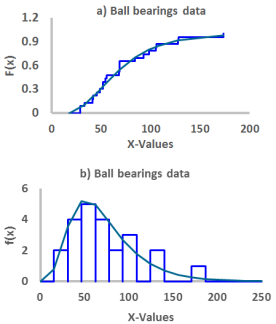
Figure 1. a) The Empirical CDF and the fitted CDF for the data. b) The Histogram and the fitted PDF for the data.
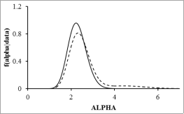
Figure 2. The posterior densities of alpha, the kernel (solid line) and the gamma (dashed line).
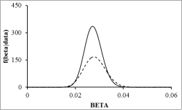
Figure 3. The posterior densities of beta, the kernel (solid line) and gamma (dashed line).
Table 1. The Bayes estimators () for the parameters and for different Priors and the Mean Square Errors (MSE), Mean Percentage Errors (MPE) under Squared Error Loss (SELF) and LINEX Loss functions (LLF) with , ( The upper row for , the lower row for ).
Table 2. The Mean Square Errors (MSE) and the Mean Percentage Errors (MPE) for the parameter ![]() for different Priors, for and under the Squared Error Loss (SELF) and LINEX Loss Functions (LLF) with .
for different Priors, for and under the Squared Error Loss (SELF) and LINEX Loss Functions (LLF) with .
Table 3. The Mean Square Errors (MSE) and the Mean Percentage Errors (MPE) for the parameter for different priors, for and under the Squared Error Loss (SELF) and LINEX Loss Functions (LLF) with .
Table 4. The Mean Square Errors (MSE) and the Mean Percentage Errors (MPE) for the parameters and for different priors, for and under the LINEX Loss Functions (LLF) with .
Information


