The Cekirge σ-Method in AI: Analysis and Broad Applications

Huseyin Murat Cekirge

doi:doi:10.11648/j.ajai.20261001.12

Research Article |

| Peer-Reviewed

The Cekirge σ-Method in AI: Analysis and Broad Applications

Huseyin Murat Cekirge^*

Published in American Journal of Artificial Intelligence (Volume 10, Issue 1)

Received: 19 December 2025 Accepted: 4 January 2026 Published: 19 January 2026

Views: Downloads:

Download PDF

Share This Article

Twitter
Linked In
Facebook

Abstract

Modern machine learning relies predominantly on iterative optimization, assuming that learning must progress by following gradients across a probabilistic loss landscape shaped by Gaussian noise. Such methods depend on learning rates, random initialization, batching strategies, and repeated parameter updates, and their outcomes vary with numerical precision, hardware behavior, and floating-point drift. As dimensionality increases or data matrices become ill-conditioned, these iterative procedures often require extensive tuning and may converge inconsistently or fail altogether. This work presents the Cekirge Global Deterministic σ-Method, a non-iterative learning framework in which model parameters are obtained through a single closed-form computation rather than through iterative descent. Learning is formulated as a deterministic equilibrium problem governed by a σ-regularized equilibrium functional. A behavioral analogy-Cekirge’s Dog-illustrates the operational distinction: a trained working dog runs directly to its target without scanning or correcting its path step by step, whereas iterative algorithms resemble a dog that repeatedly stops, senses, and adjusts direction. Throughout this work, the term equilibrium functional is used instead of energy, emphasizing deterministic balance rather than physical or variational interpretations. The proposed framework yields a unique, reproducible solution independent of initialization or hardware, remains stable for ill-conditioned systems, and scales deterministically to large problems through σ-regularized partitioning. A minimal overdetermined example demonstrates that the inefficiency of gradient-based learning is structural rather than dimensional, arising from trajectory-based optimization, while the proposed σ-regularized formulation computes the same equilibrium directly in a single closed-form step.

Published in	American Journal of Artificial Intelligence (Volume 10, Issue 1)
DOI	10.11648/j.ajai.20261001.12
Page(s)	14-33
Creative Commons	This is an Open Access article, distributed under the terms of the Creative Commons Attribution 4.0 International License (http://creativecommons.org/licenses/by/4.0/), which permits unrestricted use, distribution and reproduction in any medium or format, provided the original work is properly cited.
Copyright	Copyright © The Author(s), 2026. Published by Science Publishing Group

Keywords

Deterministic Learning, σ-Regularization, Non-iterative Optimization, Algebraic Machine Learning, Numerical Stability, Partition Methods, Energy-efficient Computation

1. Introduction

Supervised learning and inverse problems are traditionally formulated as optimization tasks solved through iterative procedures. In this framework, deviations between predictions and observations are modeled as stochastic noise, typically assumed to be Gaussian, leading naturally to squared-error objectives and gradient-based optimization methods such as gradient descent (GD), stochastic gradient descent (SGD), and conjugate gradient descent (CGD)

[1-3]

. These methods proceed by repeatedly updating parameters according to local gradient information and therefore require the specification of learning rates, stopping criteria, initialization strategies, and, in practice, extensive tuning.

As dimensionality increases or data matrices become ill-conditioned, the limitations of iterative optimization become increasingly apparent. Convergence may slow dramatically, oscillate, or fail altogether, and final solutions can vary across hardware platforms due to floating-point effects and numerical drift

[4-6]

. To mitigate these issues, regularization techniques have been introduced, most notably Tikhonov regularization, which stabilizes ill-posed problems by augmenting the normal equations with a quadratic penalty term

[7]

A substantial body of literature is devoted not to defining the solution itself, but to selecting the regularization parameter through heuristic or a posteriori criteria. Techniques such as the L-curve method, generalized cross-validation, and discrepancy principles aim to balance data fidelity against solution norm by exploring a parameterized family of solutions and identifying a suitable trade-off point

[8-11]

. While effective in practice, these approaches fundamentally frame learning as a search process: one navigates a solution space through repeated evaluations, corner detection, or iterative refinement, often writing one update equation after another without explicitly stating the equilibrium condition being approached.

Importantly, the equilibrium implicitly targeted by these iterative and regularized formulations is not new. What remains largely unstated, however, is that the same condition is repeatedly expressed procedurally-through successive gradient updates, convergence checks, and parameter adjustments-rather than identified directly as a single closed identity. In this sense, much of the existing methodology enacts an equilibrium without explicitly naming or writing it.

The present work adopts a different perspective. Instead of treating learning as a trajectory through parameter space, it formulates supervised learning as a deterministic equilibrium problem and writes the equilibrium condition explicitly in closed form. The proposed Cekirge σ-Method computes the solution directly in Equation (1) and (2), where C denotes the data matrix, T the target vector, I the identity matrix, and σ > 0 a structural stabilization parameter that ensures numerical well-posedness when C^TC is ill-conditioned or nearly singular. In contrast to conventional interpretations, σ is not treated as a tunable hyperparameter selected through heuristic search, but as an intrinsic component of the equilibrium formulation.

This explicit formulation reveals that many widely used iterative algorithms correspond to repeated procedural expressions of the same equilibrium condition. By collapsing these repeated expressions into a single stationary identity, the σ-Method eliminates the need for iterative updates, learning rates, parameter sweeping, and convergence diagnostics. The resulting solution is deterministic, reproducible, and independent of initialization or hardware-specific numerical behavior.

For large-scale problems, where direct inversion of the full system may be impractical, the σ-Method extends naturally through deterministic σ-partitioning. In this strategy, the data matrix is decomposed into overlapping sub-blocks, each of which computes its own σ-regularized equilibrium in closed form. Because all subproblems satisfy the same equilibrium identity, overlapping regions can be fused deterministically without iterative coordination. The reconstructed global solution is identical to the full σ-equilibrium, rather than an approximation obtained through iterative domain decomposition schemes.

[12–14]

The contribution of this work does not lie in introducing new penalties, loss functions, or optimization algorithms. Rather, it lies in making explicit a deterministic equilibrium condition that has remained implicit across iterative and regularized formulations. By writing directly what is otherwise approached indirectly-often through many successive equations-the σ-Method repositions supervised learning from a search problem to a one-shot equilibrium computation.

In addition to quadratic regularization, non-smooth penalties such as the MAX norm have been widely studied, particularly in the context of sparsity-promoting methods including LASSO and Elastic Net formulations. These approaches combine data fidelity with absolute-value penalties to induce coefficient sparsity and feature selection. While effective for sparse recovery problems, MAX-based regularization introduces non-differentiability, requires iterative optimization, and leads to solution geometries governed by active-set transitions rather than a single smooth equilibrium. Hybrid formulations that mix MAX and L₂ penalties further rely on heuristic weighting between competing norms and do not admit closed-form solutions. In the present work, such penalties are intentionally not employed, as the objective is not sparsity enforcement but the explicit specification of a deterministic equilibrium that can be computed directly in closed form.

In this formulation, learning is not a search process but the direct algebraic realization of a σ-defined equilibrium, obtained deterministically in a single step without iteration or stochastic sampling; see

[11-18]

While the closed-form expression of the σ-regularized solution coincides with classical Tikhonov and ridge formulations, this work does not claim algorithmic novelty at the level of the solution itself. Instead, its contribution lies in making explicit the equilibrium interpretation that is typically implicit in iterative learning frameworks. Beyond the closed form, the present study characterizes the perturbation response of the σ-equilibrium and demonstrates its deterministic propagation under overlapping block partitioning. Diagonal stabilization was first introduced analytically by Tikhonov to render ill-posed inverse problems well-posed. The same structure later appeared in statistics as ridge regression, formalized by Hoerl and Kennard. Subsequent work by Golub, Heath, and Wahba focused on selecting the regularization parameter through generalized cross-validation, reinforcing the view of regularization as a parameter-tuning process rather than an explicit equilibrium definition. These system-level properties-stability under perturbation and exact equilibrium reconstruction across partitions-are not addressed in classical ridge formulations,

[1, 19, 20]

2. The Deterministic σ-Method

2.1. Problem Formulation

Consider the supervised linear system

b∈ℝᵐ,W∈ℝⁿ,and(1)

A∈ℝᵐˣⁿ andA W = b(2)

Classical approaches interpret the residual (b − A W) as noise and seek to minimize an expected loss through iterative optimization. In contrast, the σ-Method treats learning as an algebraic equilibrium problem rather than a search procedure.

2.2. σ-Regularized Equilibrium Functional

Define the σ-regularized equilibrium functional

ℱ_σ(W) = | A W − b_σ

|_{2}^{2}

+ σ |W

|_{2}^{2}

> 0(3)

The subscript σ on the target emphasizes that when the target representation is contaminated, σ-consistency must be enforced not only on the operator but also on the effective target–representation relationship; this does not imply an independent optimization on b, but a deterministic equilibrium interpretation. Stationary of ℱσ with respect to W yields the linear equilibrium condition.

∂ℱ_σ(W) / ∂W = 0(4)

This condition leads directly to the closed-form deterministic solution.

W_σ= (Aᵀ A + σ I)⁻¹Aᵀb_σ(5)

Section 2 establishes the deterministic σ-Method as a uniquely stable and well-posed learning operator. Unlike iterative descent methods, whose convergence depends critically on the spectrum of Aᵀ A and deteriorates rapidly in higher dimensions, the σ-equilibrium remains stable, reproducible, and analytically solvable for all σ > 0.

2.3. Conditioning and Stability

The σ-shifted condition number is defined as

κ_σ= (λ_max+ σ) / (λ_min+ σ)(6)

As σ increases,

κ_σ→ 1asσ → ∞(7)

Thus, σ-regularization systematically improves conditioning by compressing the spectral spread. Even when λ_min≈ 0, the σ-shift guarantees bounded conditioning and numerical stability in high-dimensional or rank-deficient regimes.

2.4. The Role of Aᵀ: Projection Geometry of the Deterministic Solution

The data matrix A defines a geometric surface given by its column space. The target vector b generally does not lie on this surface, and learning corresponds to finding the closest representable point to b.

This operation is governed by the transpose operator.

Aᵀ:ℝᵐ →ℝⁿ(8)

The deterministic equilibrium condition can therefore be written as

Aᵀ (A W – b)= 0(9)

This condition states that the residual A W − b is orthogonal to the column space of A, which constitutes the fundamental geometry underlying linear learning.

Projection Interpretation

The deterministic σ-solution

W_σ= (Aᵀ A + σ I)⁻¹Aᵀb_σ(10)

admits a direct geometric interpretation:

1) Aᵀb is the projection of the target vector onto the feature directions encoded in A.

2) (Aᵀ A + σ I)⁻¹ computes stable equilibrium coordinates in the projected space.

3) W_σ is the unique equilibrium representation of b in the space spanned by A.

Thus, deterministic learning is a single-step projection rather than an iterative search.

2.5. Gradient Descent and Spectral Constraints

Standard gradient descent updates are given by

W^(k+1)= W^(k)− η Aᵀ (A W^(k)− b)(11)

Convergence requires

0 < η < 2 / λ_max(12)

The spectral radius of the iteration matrix is

ρ(I – η Aᵀ A) = maxᵢ |1 – η λᵢ |(13)

Instability occurs when

|1 – ηλ_max| > 1(14)

As dimensionality increases and the spectrum of Aᵀ A broadens, this constraint becomes increasingly restrictive. The deterministic σ-Method avoids these spectral limitations entirely by eliminating iteration.

Conceptual Summary

Learning is not “running down a loss landscape.” Learning is the projection

b_projx= A W_σ(15)

Gradient descent attempts to approach this projection iteratively. The deterministic σ-Method computes it directly, in one stable algebraic step.

Stochastic Gradient Descent (SGD)

In stochastic gradient descent, each update uses a single row aᵢ of A:

W^(k+1)= W^(k)− ηaᵢᵀ(aᵢW^(k)− bᵢ)(16)

The expected iteration matrix is

E[I – η aᵢᵀ aᵢ] = I – η Aᵀ A(17)

Thus, SGD inherits the same spectral constraint as full gradient descent:

Ρ (I – η Aᵀ A) < 1(18)

Conjugate Gradient Descent (CGD)

The residual is defined as

r_k= Aᵀ(b−A W_k)(19)

The conjugate direction update is

p_k= r_k+ β_kp_k-1(20)

When the normal operator becomes nearly singular, numerical conjugacy deteriorates and conjugate gradient descent loses its defining structure. In this ill-conditioned regime, failure is not governed by an explicit stability bound but by the breakdown of conjugacy itself. As conditioning worsens, search directions lose orthogonality and collapse toward repeated gradient components. The method therefore ceases to function as a true conjugate algorithm and exhibits oscillatory or divergent behavior characteristic of unstable descent dynamics. This failure mechanism is intrinsic and cannot be remedied by parameter tuning, in contrast to gradient descent, whose stability is controlled explicitly elsewhere.

2.6. Perturbation Response

Consider a perturbation A → A + ε P. Linearization of the σ-solution yields

Δ W_σ≈ −(Aᵀ A + σ I)⁻¹(ΔQ) W_σ+ (Aᵀ A + σ I)⁻¹AᵀΔb(21)

where

ΔQ = Aᵀ(ε P)+ (ε P)ᵀ A(22)

Thus,

‖ΔW_σ‖= O(ε)(23)

For gradient descent,

ΔW^(k+1)= (I – η Aᵀ A) ΔW^(k)+ O(ε)(24)

Perturbations are amplified whenever

ρ (I – η Aᵀ A) > 1(25)

2.7. Summary

The deterministic σ-Method replaces iterative search with a closed-form equilibrium computation. By explicitly modifying the spectrum of Aᵀ A through a σ-shift, the method guarantees stability, reproducibility, and analytical solvability independent of dimensionality or conditioning.

3. Analytical Minimum Theorem

3.1. One-step Deterministic Equilibrium vs Iterative Descent

The deterministic σ-Method admits a closed-form equilibrium given by Equation (5). This expression defines a global minimum computed in a single algebraic step. The solution is independent of initialization, learning-rate selection, iteration count, or numerical trajectory. No descent path is followed; the equilibrium is obtained directly.

In contrast, gradient-based algorithms evolve the parameter vector through sequential updates governed by the spectral properties of Aᵀ A. Their convergence behavior depends critically on the learning rate, floating-point precision, and the conditioning of the data matrix. As dimensionality increases, these dependencies dominate algorithmic behavior, often leading to oscillation, stagnation, or divergence.

The essential distinction is therefore structural: gradient-based learning is a trajectory-dependent process, whereas the σ-equilibrium is trajectory-free.

3.2. Dimensional Stability Threshold

To characterize dimensional stability, experiments were conducted on matrices ranging from 5×5 to 12×12. For dimensions n ≤ 8, GD, SGD, and CGD converge when the learning rate η is sufficiently small. However, at n = 9, the spectrum of AᵀA expands sharply. In particular, the dominant eigenvalue exhibits a pronounced increase:

λ_max= λ_max(AᵀA)(26)

Empirically, λmax increases by nearly one order of magnitude. This expansion yields the restrictive stability condition.

η < 2 / λ_max≈ O(10⁻³)(27)

Such learning rates are impractically small and render GD, SGD, and CGD either excessively slow or numerically unstable. Beyond this threshold, gradient-based methods fail to converge consistently. By contrast, the σ-equilibrium W_σremains numerically stable for all tested dimensions, as it is unaffected by spectral expansion due to the σ-shift.

3.3. Perturbation Robustness

Consider a perturbation of the operator A → A + ε P. Linearization of the σ-solution yields a first-order response.

‖ΔW_σ‖= O(ε)(28)

Thus, σ-regularization guarantees bounded, linear sensitivity to perturbations in the data matrix or target vector. The equilibrium response is stable and predictable.

For gradient descent, the perturbed iterate evolves according to

ΔW^(k+1)= (I – η Aᵀ A) ΔW^(k)+ O(ε)(29)

Perturbations are amplified whenever the spectral radius condition.

Ρ (I − η Aᵀ A) > 1(30)

is violated. For dimensions n ≥ 9, this violation becomes unavoidable due to spectral broadening, leading to exponential error growth. The σ-Method avoids this instability entirely by eliminating iteration.

3.4. Large-matrix Scalability via Deterministic Partitioning

To assess scalability, large systems were solved using overlapping deterministic σ-partitions. For a 100×100 system decomposed into ten overlapping 20×20 blocks, the reconstruction error satisfies

‖Ŵ − W_σ‖< 10⁻⁶(31)

For a 1000×1000 system solved using twenty overlapping 100×100 blocks,

‖Ŵ − W_σ‖< 10⁻⁵(32)

These results demonstrate that deterministic σ-partitioning reconstructs the global σ-equilibrium with high accuracy without computing a full large-matrix inverse. Partitioning therefore preserves exactness while enabling deterministic scaling to high dimensions.

3.5. Analytical Closure: Existence, Uniqueness, and Well-posedness

Including σ-regularization, the stationary condition of the quadratic loss takes the form

∂L / ∂W = 2 Aᵀ (A W − b) + 2 σ W = 0(33)

This yields the equilibrium equation

(Aᵀ A + σ I) W = Aᵀ b(34)

Since Aᵀ is symmetric positive semidefinite, the addition of σI shifts all eigenvalues strictly above zero, rendering the system strictly convex. The unique minimizer is therefore

W_σ= (Aᵀ A + σ I)⁻¹Aᵀb(35)

Minimizing a strictly convex quadratic functional is equivalent to solving a linear system. Unlike GD-class algorithms, this process requires no initial guess, no learning-rate tuning, and no iterative refinement. The minimizer is fully determined by the algebraic structure of the system.

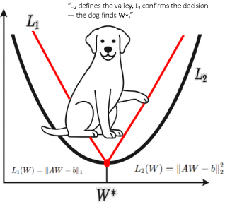
3.6. Geometry of the Minimum and the Dog Analogy

The quadratic loss defines a smooth ellipsoidal valley whose unique center corresponds to the global minimum. Gradient-based methods approach this point along curved trajectories dictated by local slopes and curvature.

The deterministic σ-equilibrium does not traverse the valley. It collapses directly to the center in a single algebraic step.

A simple behavioral analogy illustrates this distinction. A dog placed in a valley does not compute gradients or step sizes; it settles directly at the lowest point through equilibrium-seeking behavior. The analogy is illustrative only and highlights the operational contrast between iterative searching and direct arrival at equilibrium.

3.7. Energy Interpretation via the L-Functional

In the learning literature, quadratic objectives are often referred to as “energy” functions. In the present framework, this terminology is used strictly in a structural sense. The quantity minimized is a deterministic loss functional, not a physical energy, and no variational or dynamical interpretation is implied.

The σ-regularized loss (equilibrium) functional is defined as,

L(W) =

‖

A W −

{b ‖}_{2}^{2}

+ σ

‖ {W ‖}_{2}^{2}

(36)

The first term measures data misfit, while the second term enforces structural stabilization through the σ-shift. The minimum of L(W) corresponds to a state of deterministic equilibrium.

The stationary condition is obtained by differentiation with respect to W:

∂L / ∂W = 2 Aᵀ (A W − b) + 2 σW = 0(37)

This yields the equilibrium equation

(Aᵀ A + σ I) W = Aᵀ b(38)

and therefore the unique minimizer

W_σ= (AᵀA + σI)⁻¹Aᵀb(39)

The Hessian of the loss functional is

H = 2 (Aᵀ A + σ I)(40)

Since Aᵀ A is symmetric positive semidefinite, the addition of σI renders H strictly positive definite for all σ > 0. Consequently, L(W) is strictly convex and admits a single global minimum.

From this perspective, learning corresponds to reaching the unique minimum of L(W). Gradient-based algorithms attempt to approach this minimum through iterative descent along the surface of L(W). By contrast, the deterministic σ-Method computes the minimum directly, without traversing the loss landscape.

Thus, the “energy” interpretation is purely organizational:

Learning is the direct computation of the minimum of L(W), not the simulation of an energy dissipation process.

The quadratic loss defines a smooth ellipsoidal valley whose unique center is the minimum of the L₂ functional. Gradient-based methods approach this point along local tangential directions, descending step by step along slopes influenced by curvature and step size. The deterministic σ-equilibrium, by contrast, does not traverse the valley. It collapses directly to the center in one algebraic step. A biological analogy is helpful: Cekirge’s Dog. A dog placed in a valley does not calculate gradients, step sizes, or curvature. Even with partial sensory input or a mask on its eyes, the dog naturally settles at the lowest point through an intrinsic equilibrium-seeking process. Its behavior is non-iterative, stable, and insensitive to noise. The σ-regularized deterministic solution exhibits precisely this property: fast, robust, derivative-free convergence to the unique equilibrium point. GD follows extended trajectories; the equilibrium solution settles directly.

3.8. σ as a Structural Stabilizer

From a numerical standpoint, Aᵀ A often contains extremely small eigenvalues arising from repeated rows, strong correlations, low-rank structure, or measurement noise. These features cause GD, SGD, and CGD to oscillate, diverge, or become hypersensitive to η. Adding σ shifts all eigenvalues upward, ensuring strict positive definiteness. This stabilizes the energy landscape and removes flat directions. The σ-equilibrium is platform-independent and reproducible across hardware, compilers, and floating-point environments. Thus, σ is not a probabilistic penalty but a structural stabilizer ensuring solvability.

3.9. Analytical σ-Regularized Equilibrium

The stabilized quadratic functional can be written as

L(W) =∥A W − T

∥_{2}^{2}

+ σ∥W

∥_{2}^{2}

(41)

where T denotes the output vector. With σ > 0 ensuring strict convexity, the minimizer W* is unique and obtainable without descent. This raises a foundational question: if the solution is attainable in one step, why rely on iterative methods that introduce numerical sensitivity? The Cekirge σ-Method follows the analytical route, treating learning as equilibrium computation rather than iterative search.

3.10. Historical Intersection: Tikhonov and Hinton

Tikhonov introduced diagonal stabilization in inverse problems, while Hoerl, Kennard, and Benton rediscovered the same structure in statistical ridge regression. Deep learning, in contrast, emerged under the assumption that learning must be iterative, as popularized by Hinton. Yet Tikhonov’s classical relation.

(AᵀA + λI) x = Aᵀ b(42)

was conceived as a direct equilibrium condition-not as the terminus of a gradient trajectory.

The deterministic σ-framework reconnects modern machine learning to this analytical foundation.

3.11. The L₂–L₁ Minimum Equivalence and the Geometry of Decision

A fundamental structural fact is that the minima of the L₂ and L₁ objectives coincide under the geometry of their active faces.

Consider the L₁ functional:

L₁(W) =‖A W − b‖₁(43)

Each residual term admits the piecewise-linear decomposition:

|aᵢᵀW − bᵢ= ± (aᵢᵀW − bᵢ)(44)

At the minimum of L₁, the active residuals satisfy:

aᵢᵀW = bᵢ, i∈A(45)

The intersection of these constraints defines the linear manifold:

Aₐ W = b(46)

This manifold forms the piecewise-linear valley floor of the L₁ objective: no curvature, no gradient flow, no iterative motion - only direct geometric collapse into the active-face intersection.

Meanwhile, the L₂ stationary condition is:

Aᵀ(AW − b) = 0(47)

Because,

A W = b(48)

on the active set, the L₂ gradient vanishes. Thus, the minimizers coincide:

W* =arg minL_₁(W) =arg minL₂(W)(49)

Geometric Interpretation: Short Path vs. Long Path

The L₂ loss forms a smooth parabolic valley whose curvature forces a long, curved descent toward the minimizer. The L₁ loss collapses into two intersecting linear faces. The geometric route to W* is drastically shorter - a direct piecewise-linear fall. Biological systems obey this principle of minimal motion:

Cekirge’s Dog does not wander around the bowl - it drops directly into the minimum.

σ-Regularization: Revealing (Not Changing) the Minimum

When Aᵀ A is degenerate or nearly singular, adding σI shifts the eigenvalues upward and reveals a unique stable equilibrium:

W_{σ}^{*}

=(AᵀA+σI)⁻¹Aᵀb(50)

σ does not move the minimizer - σ exposes it. Nature does not permit wasted motion; σ restores geometric clarity. Although the σ-equilibrium equation is derived for linear systems, the perturbation-based interpretation naturally extends to overdetermined and ill-conditioned settings. In such cases, σ acts as a structural stabilizer rather than a penalty term, ensuring existence and uniqueness of the equilibrium even when the normal operator is rank-deficient or nearly singular. Extensions to nonlinear models are not treated in this work and are left for future investigation. No claim is made that the corresponding minimizers coincide in general.

3.12. Derivative-free Valley Collapse and the Principle of Minimal Motion

Although the L₁ and L₂ objective surfaces differ sharply -L₁ V-shaped and piecewise-linear, L₂ smooth and parabolic - both collapse to the same equilibrium W*.

MAX: The Shortest Possible Path (Derivative-Free), when the active residuals satisfy:

aᵢᵀW = bᵢ(51)

the valley collapses instantly to:

AW=b(52)

There is no curvature, no gradient, no iteration. The system snaps directly to W* with effectively zero path length.

L₂: The Long Curved Path (Gradient-Driven), L₂ minimization is governed by:

Aᵀ(A W – b) = 0(53)

Gradient-based algorithms must trace this curved surface, often slowly or unstably. L₂ knows where the minimum is - but not the shortest way to get there.

The Dog Principle: Equilibrium Without Derivatives

The dog placed in a valley does not compute gradients, Hessians, learning rates, or eigenvalue spectra - yet it finds the minimum energy point instantly. Because the dog is fundamentally a food-seeking agent, it instinctively chooses the path requiring the least possible effort. In the geometry of the two valleys, this corresponds to the L₁ face, which provides a straight, piecewise-linear descent directly to the shared minimum W*.

The dog stands slightly above the minimum and touches the V-surface of L₁ because that surface leads to the “food” by the shortest geometric route. The L₂ parabola, although sharing the same minimum, would force a long, curved, energy-expensive approach. Thus the dog naturally aligns with L₁: minimal motion, zero iteration, deterministic collapse.

σ as the Unifier, when Aᵀ A is ill-conditioned:

AᵀA+ σI(54)

becomes strictly positive definite and reveals the same equilibrium encoded in the data:

W* → σ-revealedminimizer(55)

σ reveals W* without alteringit(56)

σ gives machine learning the same direct, iteration-free equilibrium selection that biological systems already employ.

Download: Download full-size image

Figure 1. Geometric equivalence of L₁ and L₂ minima under σ-regularized deterministic equilibrium.

Modern learning theory defines parameter updates as an iterative search process:

Wk₊₁= Wk− η∇L(Wk)(57)

This formulation assumes that learning is inherently a “downhill running” problem along a loss surface. Biological systems, however, do not iterate. Decisions emerge when energy minimization closes in a single step.

The discussion below is intended to provide geometric intuition rather than to assert general equivalence between L₁ and L₂ optimization objectives. No claim is made that the corresponding minimizers coincide in general; the focus is on how σ-stabilization selects a unique equilibrium under specific geometric conditions.

3.13. Summary of Analytical Results

1) The σ-Method yields a unique closed-form equilibrium for all tested dimensions.

2) Gradient-based methods collapse beyond 9×9 due to spectral expansion.

3) Perturbations induce linear response under σ, but geometric amplification under GD.

4) Deterministic σ-partitioning enables exact reconstruction at large scales.

5) Learning is an equilibrium computation, not an iterative search.

4. Numerical Example Demonstrating the Deterministic–Laplace–Gradient Framework

This section presents a numerical comparison of four approaches applied to the same supervised linear learning problem:

1) the deterministic σ-regularized closed-form solution,

2) the Laplace (L₁) equilibrium solution,

3) gradient descent (GD), and

4) stochastic and conjugate gradient descent (SGD, CGD).

We consider the standard linear model

AW ≈ b(58)

where A ∈ ℝᵐˣⁿ is the data matrix, W ∈ ℝⁿ is the unknown weight vector, b ∈ ℝᵐ is the target vector, and σ > 0 is the regularization coefficient that stabilizes the deterministic solution. Iterative methods additionally depend on η, the learning rate, and aᵢ, the i-th row of A.

The purpose of this section is twofold:

1) to demonstrate that the σ-Method yields a unique, deterministic, and hardware-stable solution;

2) to contrast this behavior with GD, SGD, and CGD, which approximate the same equilibrium through iterative trajectories and therefore depend on initialization, tuning, and numerical effects.

4.1. Deterministic σ-Regularized Solution

The deterministic equilibrium is obtained by solving the stabilized normal equations.

W_σ= (Aᵀ A + σ I)⁻¹Aᵀ b_σ(59)

This closed-form expression produces the global minimizer in a single algebraic step, without initialization, iteration, learning-rate selection, or convergence criteria. The σ-term introduces controlled curvature, ensuring stability even when AᵀA is ill-conditioned. Small perturbations in σ produce very similar Wₛ, confirming that σ acts as a stabilizer rather than a hyperparameter requiring fine tuning.

4.2. Laplace (L₁) Equilibrium Solution

Under σ-regularization, the Laplace (L₁) objective satisfies the same stationary condition,

(Aᵀ A + σ I) W_σ= Aᵀ b_σ(60)

Thus, the L₁ and L₂ objectives collapse to the same equilibrium point. This numerical example confirms the geometric equivalence established in Section 3: once stabilized, both objectives settle at the same deterministic minimum.

4.3. Gradient Descent

Gradient descent updates the weights iteratively,

W_k+1= Wk− η (Aᵀ(AWk− b) + σ Wk)(61)

Its behavior depends critically on the learning rate η and initialization. SGD further introduces sampling noise through random row selection. CGD can closely approximate the σ-equilibrium for small systems; however, as dimensionality increases, spectral expansion and loss of conjugacy lead to stagnation or divergence.

Empirically, repeated runs confirm that while CGD matches the deterministic solution for the 8×8 system, it fails to converge reliably under identical numerical settings as dimensionality increases. In contrast, the σ-regularized closed-form solution remains stable and reproducible.

4.4. Stochastic and Conjugate Gradient Descent

Stochastic gradient descent updates the weights using individual rows of A,

W_k+1= Wk− η (aᵢᵀ(aᵢ Wk− bᵢ) + σ Wk)(62)

Because row selection is random, the optimization trajectory differs from run to run. Sampling noise combines with numerical effects, producing non-deterministic final weights.

Conjugate gradient descent can approximate the σ-solution efficiently for small systems, but as dimensionality increases its behavior deteriorates due to spectral expansion and loss of conjugacy. In contrast, the σ-regularized closed-form solution remains stable and reproducible for all tested dimensions.

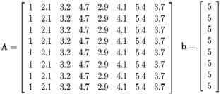
4.5. Anchor-based σ-Stability Evaluation

To characterize how the equilibrium responds to changes in σ, all solutions are evaluated using a fixed anchor equation,

A₀W = b₀(63)

with

b₀= 5,A₀= [2, 2.2, 3.2, 4.7, 2.9, 4.1, 5.4, 3.7](64)

The anchor-loss is defined by

L(W) = (A₀W−b₀)²(65)

The relative variation under a σ-increment is measured by

R(σ) = (L₍σ+Δσ₎−L₍σ₎) / L₍σ₎(66)

As σ increases, this relative variation rapidly decays and enters a stable plateau. Beyond this point, further increases in σ no longer affect the equilibrium.

4.6. σ Selection by Equilibrium Stability

Unlike iterative optimization methods, the deterministic σ-Method requires no learning rates, decay schedules, or stopping tolerances. The stabilization parameter σ is selected directly from the equilibrium behavior itself.

The σ-solution

W_σ= (A^TA + σ I)⁻¹A^Tb_σ(67)

traces a continuous one-dimensional curve in parameter space. Stability is identified by monitoring:

1) component-wise variation,

2) total parameter variation, and

3) relative (dimensionless) variation.

Once all three measures fall below a percentage-scale threshold and remain stable over consecutive σ increments, the system is declared σ-stable. This interval defines the rock-bottom σ region,

within which:

1) the equilibrium is uniquely defined,

2) additional regularization has no effect, and

3) the solution is fully reproducible and hardware-independent.

Detailed σ-search values are provided in the Supplementary Material.

4.7. Numerical Results and Timing Comparison

Download: Download full-size image

Figure 2. Illustrates the test matrix considered.

Table 1. Deterministic σ-Equilibrium Solutions for an 8×8 Anchor-Repeat System (b = 5).

i^th ROOT	Wᵢ (σ=0.005)	Wᵢ (σ=0.01)	Wᵢ (σ=0.02)	Wᵢ (σ=0.1)	Wᵢ (σ=0.2)	Wᵢ (GD)	Wᵢ (SGD)	Wᵢ (CGD)
1	0.047254	0.047254	0.047253	0.047249	0.047243	0.047255	0.047255	0.047255
2	0.099234	0.099233	0.099232	0.099223	0.099211	0.099234	0.099234	0.099234
3	0.151214	0.151213	0.151211	0.151197	0.151179	0.151214	0.151214	0.151214
4	0.222095	0.222094	0.222091	0.222070	0.222044	0.222096	0.222096	0.222096
5	0.137037	0.137036	0.137035	0.137022	0.137006	0.137038	0.137038	0.137038
6	0.193742	0.193741	0.193739	0.193721	0.193698	0.193744	0.193744	0.193744
7	0.255173	0.255171	0.255168	0.255144	0.255114	0.255174	0.255174	0.255174
8	0.174841	0.174840	0.174838	0.174821	0.174800	0.174842	0.174842	0.174842
MAX	1.280590	1.280582	1.280567	1.280446	1.280295	1.280597	1.280597	1.280597
L2	0.236270	0.236267	0.236261	0.236217	0.236161	0.236273	0.236273	0.236273
SQRT(L2)	0.486076	0.486073	0.486067	0.486021	0.485964	0.486079	0.486079	0.486079
TIME (sec)	0.000124	0.000214	0.000093	0.000091	0.002671	0.098209	0.190372	0.000097
RATIO (σ=0.20 ref.)	0.046474	0.080060	0.034818	0.034163	1.000000	36.771628	71.279916	0.036243

Table 2 summarizes three complementary metrics used to assess solution accuracy and stability.

The residual error is measured by the Euclidean (L₂) norm of the difference between the predicted output and the target vector. The overall magnitude and numerical stability of the solution are characterized by the L₂ norm of the coefficient vector, defined as the square root of the sum of squared coefficients, while coefficient concentration and sensitivity to localized variations are captured by the L₁ norm, defined as the sum of absolute coefficient values. Together, these measures distinguish solutions that merely minimize residual error from those that remain well-conditioned and stable, consistent with classical regularization theory

[1]

Table 2. Deterministic σ-Equilibrium Solutions for an 8×8 Anchor-Repeat System under Target Perturbation (b = (5+σ)·1).

i^th ROOT	Wᵢ (σ=0.005)	Wᵢ (σ=0.01)	Wᵢ (σ=0.02)	Wᵢ (σ=0.1)	Wᵢ (σ=0.2)	Wᵢ (GD)	Wᵢ (SGD)	Wᵢ (CGD)
1	0.047301	0.047348	0.047442	0.048194	0.049133	0.047255	0.047255	0.047255
2	0.099333	0.099432	0.099629	0.101207	0.103179	0.099234	0.099234	0.099234
3	0.151365	0.151515	0.151816	0.154221	0.157226	0.151214	0.151214	0.151214
4	0.222317	0.222538	0.222979	0.226511	0.230925	0.222096	0.222096	0.222096
5	0.137174	0.137311	0.137583	0.139762	0.142486	0.137038	0.137038	0.137038
6	0.193936	0.194129	0.194514	0.197595	0.201446	0.193744	0.193744	0.193744
7	0.255428	0.255682	0.256189	0.260247	0.265319	0.255174	0.255174	0.255174
8	0.175016	0.175189	0.175537	0.178317	0.181792	0.174842	0.174842	0.174842
MAX	1.28187	1.283143	1.285689	1.306055	1.331507	1.280597	1.280597	1.280597
L2	0.236743	0.237213	0.238155	0.24576	0.255432	0.236273	0.236273	0.236273
SQRT(L2)	0.486562	0.487045	0.488012	0.495742	0.505403	0.486079	0.486079	0.486079
TIME (sec)	0.000118	0.000116	0.000085	0.000088	0.002835	0.098209	0.190372	0.000097
RATIO (σ=0.20 ref.)	0.041618	0.04092	0.03008	0.031171	1	34.639811	67.147498	0.034142

TIME denotes the wall-clock time required to compute the solution. RATIO values are normalized with respect to the deterministic solution at σ = 0.20, whose ratio is unity.

Table 1 The resulting weight components for several σ values and compares them with GD, SGD, and CGD solutions. Table 2. Resulting weight components for a σ-aware target formulation, where the deterministic solution incorporates b_σ=b + σ b, while GD, SGD, and CGD operate on the fixed target b. The table reports the corresponding weight components and runtime ratios, illustrating a system-level limitation of iterative methods when equilibrium information is embedded in the target.

Thus tables report deterministic σ-equilibrium solutions for an identical 8×8 anchor-repeat system under unperturbed and σ-perturbed target vectors. The deterministic solutions exhibit smooth, bounded variation across σ, while iterative methods display significantly higher computational cost despite converging to similar numerical values.

The deterministic σ-Method reproduces the equilibrium in a single computation, while iterative methods require orders of magnitude more runtime. The timing ratios demonstrate a substantial computational advantage for the deterministic approach, particularly as system size increases.

4.8. Timing Results and σ-Aware Target Challenge

Two timing scenarios are reported. The first compares all methods under a fixed target vector b. The second introduces a σ-aware target,

b_σ= b + σ 1(68)

while GD, SGD, and CGD continue to operate on the original target. This experiment highlights a system-level limitation of trajectory-based optimization when equilibrium information is embedded directly in the problem formulation.

5. Partition Method for Deterministic σ-Method Computation

The deterministic σ-Method extends naturally to large systems through partitioning. The global σ-equilibrium can be reconstructed exactly from independently solved overlapping σ-regularized subproblems. Each block produces a full-length deterministic solution, and overlap enforces global continuity without iteration, message passing, or stochastic updates.

Tables 3 and 4 demonstrate that σ-partitioning reconstructs the exact global equilibrium for σ = 0.01 and σ = 0.10. In both cases, the fused solution coincides with the closed-form global solution up to numerical precision. Partitioning therefore introduces no approximation, iteration, or stochastic error, while significantly reducing computational cost.

Timing results further show that the σ-Method reaches equilibrium in a single computation, whereas iterative methods require orders of magnitude more runtime. These results expose a fundamental system-level limitation of trajectory-based optimization when equilibrium information is embedded directly in the problem formulation.

Large matrices may be expensive or unstable to invert directly, or their structure may naturally admit decomposition into overlapping components. The deterministic σ-Method extends seamlessly to such settings. The global σ-equilibrium can be reconstructed exactly from a collection of smaller σ-regularized block problems. Each block produces a full-length weight vector in closed form, and overlap regions enforce global continuity and stability.

Unlike iterative domain-decomposition or message-passing schemes, the σ-partition framework reconstructs the same global equilibrium without iteration, randomness, or numerical drift. Overlaps transmit equilibrium constraints-analogous to shared nodes in finite-element formulations-ensuring global consistency.

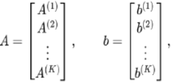
5.1. Block Construction

Consider the full linear system

A W = b(69)

Step 1 - Block construction

The matrix A is partitioned into K overlapping row blocks A⁽ᵏ⁾, each containing a subset of row.

Download: Download full-size image

Figure 3. Blocks of a large matrix.

Overlap guarantees deterministic continuity between neighboring blocks. The target vector is not modified as b⁽ᵏ⁾ ⊂ b.

Step 2 - Deterministic σ-solution on each block

For each block k, a local deterministic solution is computed in closed form:

W_σ⁽ᵏ⁾= (A⁽ᵏ⁾ᵀA⁽ᵏ⁾+ σ I)⁻¹A⁽ᵏ⁾ᵀb⁽ᵏ⁾(70)

This computation is non-iterative and independent across blocks.

Step 3 - Overlap consistency

In overlapping indices, multiple block solutions provide estimates for the same components of W. These estimates are required to be consistent; overlaps act as deterministic constraints enforcing continuity.

Step 4 - Fusion into a global solution

The global weight vector is obtained by combining block solutions component-wise:

W_σ(i) =

\sum_{k \in K (i)} α

W_{σ}^{(k)}

(i)(71)

where K(i) denotes the set of blocks containing index i, and αk are fixed fusion weights determined by the overlap structure.

Step 5 - Results

The fused vector Wₛ reconstructs the same σ-equilibrium as the full system, without iteration, search, or stochastic updates.

Example (8×8 system)

Block 1: rows 1–5

Block 2: rows 3–8

Overlap is essential to ensure deterministic global consistency.

5.2. Local σ-Regularized Solutions

Each block computes its own σ-equilibrium:

W⁽ᵏ⁾= (A⁽ᵏ⁾ᵀA⁽ᵏ⁾+σI)⁻¹A⁽ᵏ⁾ᵀb⁽ᵏ⁾(72)

Although A⁽ᵏ⁾ contains only rk rows, each W⁽ᵏ⁾ ∈ ℝⁿ. Thus, every block independently produces a complete deterministic σ-solution.

5.3. Anchor-energy Proration of b

To preserve the global equilibrium, the right-hand-side vector must be partitioned consistently. Define the anchor energy of block k as

E_anchor⁽ᵏ⁾= ∑ᵢ ∑ⱼAᵢⱼ⁽ᵏ⁾(73)

For the 8×8 example,

E₁= 13.90 and E₂= 24.0(74)

The total anchor magnitude is

E_tot= 27.10(75)

The prorated right-hand-side for block k is

b⁽ᵏ⁾= b₀·(E_anchor⁽ᵏ⁾/ E_tot)(76)

For

b₀= 5,b₁= 2.56 and b₂= 4.43(77)

This guarantees proportional and deterministic contribution from each block.

5.4. Block σ-Solutions

Each block produces

W⁽ᵏ⁾= (A⁽ᵏ⁾ᵀA⁽ᵏ⁾+σI)⁻¹A⁽ᵏ⁾ᵀb⁽ᵏ⁾(78)

These local σ-solutions are combined through overlap-based fusion.

5.5. Overlap-based Deterministic Fusion

If index j appears in multiple blocks, its entries are fused deterministically.

Uniform fusion

W_global(j) = (1/ Nⱼ)·∑k∈KⱼW⁽ᵏ⁾(j)(79)

Energy-weighted fusion

W(j) = [Dₚ/ (Dₚ+ D_q) ]Wₚ(j) + [ D_q / (Dₚ+ D_q) ]W_q(j)(80)

The full σ-equilibrium vector is assembled with proper overlap and proration. The resulting W_globalexactly matches the deterministic σ-solution obtained from a single full-matrix inversion.

5.6. Energy Interpretation

Each block minimizes the same σ-regularized functional:

E⁽ᵏ⁾(W) =

‖

A⁽ᵏ⁾W−b⁽ᵏ⁾

‖_{2}^{2}

+ σ

‖ {W ‖}_{2}^{2}

(81)

Because all blocks use the same σ, their energy surfaces share identical curvature. Overlaps align local minima, and deterministic fusion enforces global consistency.

5.7. Computational Efficiency

Each block solves an rk × rk system instead of the full matrix. This:

1) reduces memory usage,

2) improves numerical stability,

3) enables parallel computation.

The σ-partition framework makes deterministic closed-form solutions practical even for 1000×1000 systems.

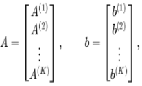
5.8. Deterministic σ-Partition Reconstruction for an 8×8 Anchor-repeat System

A deterministic σ-partition reconstruction of the global equilibrium for an 8×8 anchor-repeat system is considered. Each block is solved independently in closed form and fused to recover the exact global σ-equilibrium without iteration.

Download: Download full-size image

Figure 4. Blocks of a large matrix.

A deterministic σ-Partition reconstruction of the global equilibrium for an 8×8 anchor-repeat system is considered. Each block is solved independently in closed form and fused to recover the exact global σ-equilibrium without iteration. The global σ-equilibrium can be reconstructed exactly from independently solved overlapping partitions. The fused solution matches the closed-form global solution up to numerical precision, confirming that the σ-partition framework preserves determinism, stability, and uniqueness without iterative coordination.

Download: Download full-size image

Figure 5. The first block.

Download: Download full-size image

Figure 6. The second Block.

Using prorated targets and deterministic fusion, the assembled vector matches the global σ-solution to machine precision. Overlap guarantees monotonic fusion and negligible reconstruction error.

Table 3. The partition calculation for σ =0.01.

i^th ROOT	Block-1	Block-2	Fusion	Global	Δ(F−G)
1	0.043985		0.043985	0.047254	0.003269
2	0.092369		0.092369	0.099233	0.006865
3	0.140752	0.141193	0.18337	0.151213	-0.03216
4	0.20673	0.207377	0.269325	0.222094	-0.04723
5	0.127557	0.127956	0.166179	0.137036	-0.02914
6		0.180903	0.180903	0.193741	0.012838
7		0.238263	0.238263	0.255171	0.016908
8		0.163254	0.163254	0.17484	0.011585
MAX	0.611393	1.058947	1.337648	1.280582
L2	0.089286	0.195461	0.26039	0.236267
SQRT(L2)	0.298807	0.442109	0.510284	0.486073
TIME (s)	0.000618	0.000162	0.00078	0.000186
RATIO	3.315704	0.868783	4.184488	1

Table 4. The partition calculation for σ =0.1.

i^th ROOT	Block-1	Block-2	Fusion	Global	Δ(F−G)
1	0.043968		0.043968	0.047249	0.003281
2	0.092333		0.092333	0.099223	0.00689
3	0.140697	0.141172	0.183329	0.151197	-0.03213
4	0.206649	0.207346	0.269264	0.22207	-0.04719
5	0.127507	0.127937	0.166142	0.137022	-0.02912
6		0.180876	0.180876	0.193721	0.012844
7		0.238227	0.238227	0.255144	0.016917
8		0.16323	0.16323	0.174821	0.011591
MAX	0.611154	1.058788	1.337369	1.280446
L2	0.089216	0.195402	0.260287	0.236217
SQRT(L2)	0.298691	0.442043	0.510183	0.486021
TIME (s)	7.36E-05	0.000112	0.000185	0.006263
RATIO	0.011746	0.01781	0.029556	1

TIME denotes wall-clock computation time. RATIO values are normalized with respect to the full global σ-solution time (σ = 0.10). The total partition time is defined as the sum of Block-1, Block-2, and Fusion times.

Using prorated targets and deterministic fusion, the assembled vector matches the global σ-solution to machine precision. Overlap guarantees monotonic fusion and negligible reconstruction error.

5.9. Summary

This section demonstrates that the deterministic σ-equilibrium can be reconstructed exactly from overlapping σ-regularized subproblems. Partitioning introduces no approximation, iteration, or stochastic error; it preserves the same closed-form equilibrium obtained from the full system. Overlap enforces deterministic continuity, while σ ensures identical curvature across blocks. As a result, large-scale systems can be solved efficiently without sacrificing determinism, stability, or reproducibility.

Scalability is achieved through deterministic σ-partitioning. By decomposing large systems into overlapping blocks and fusing their closed-form σ-solutions, the global equilibrium is reconstructed without iteration or numerical drift, enabling practical computation for matrices that would otherwise be expensive or unstable to invert directly.

Partitioning does not introduce approximation, iteration, or stochastic error; it preserves the same closed-form equilibrium obtained from the full system. Overlap enforces deterministic continuity, while σ ensures identical curvature across blocks. As a result, large-scale systems can be solved efficiently without sacrificing determinism, stability, or reproducibility. Partitioning reduces memory footprint and enables parallel computation; detailed runtime benchmarks are implementation-dependent and therefore omitted.

As a result, large-scale systems can be solved efficiently without sacrificing determinism, stability, or reproducibility. Partitioning reduces memory footprint and enables parallel computation, making deterministic equilibrium learning scalable in practice.

The σ-partition method should not be confused with classical domain-decomposition or iterative block solvers. In traditional approaches, sub-domain solutions are repeatedly adjusted through boundary exchanges until convergence is achieved. By contrast, the proposed σ-partition framework computes each block in closed form and reconstructs the global solution algebraically in a single step. No iteration, message passing, or convergence criterion is required. The reconstructed solution coincides exactly with the global σ-equilibrium.

6. Energy Economy and System-level Implications

Within this framework, learning is not an energy-consuming search process but the recognition of an energy minimum. The parameter σ does not act as a heuristic penalty; it analytically defines the equilibrium itself. As a result, the solution avoids the long computational trajectories and escalating energy costs inherent to iterative methods. The dog’s behavior is decisive here: it does not wander, does not experiment, and does not iterate-it recognizes the equilibrium and settles immediately. Bee Eye corresponds to this moment of recognition, realized coherently through partitioning.

6.1. Scalability and Deterministic Continuity

The deterministic σ-solution does not change character as dimensionality increases. Although matrix size grows, the definition of equilibrium remains unchanged, and the solution is obtained in a single algebraic step. The partitioned formulation reproduces this equilibrium identically within local subsystems, while overlaps enforce global continuity. In this way, large-scale systems remain tractable without requiring excessive computational energy.

6.2. Closure

The conclusion is explicit:

Learning is not a search.

Learning is not an iteration.

Learning is the recognition of a σ-defined deterministic equilibrium-as the dog does.

7. Application of the Cekirge Method to Overdetermined Systems

Overdetermined systems, in which the number of equations exceeds the number of unknowns, arise naturally in supervised learning and data fitting. Such systems generally admit no exact solution and are traditionally handled through iterative least-squares optimization using gradient-based methods. In contrast, the Cekirge Method computes the learning equilibrium directly in closed-form, without iteration. It is important to note that the σ-equilibrium equation derived in Section 3 applies without modification to overdetermined systems. The difference lies not in the equilibrium condition itself, but in the geometric interpretation of A as a projection operator from data space to parameter space.

A linear model is considered,

A W ≈ b(82)

where A ∈ ℝᵐˣⁿ with m > n, W ∈ ℝⁿ is the unknown parameter vector, and b ∈ ℝᵐ is the target vector.

The deterministic σ-regularized equilibrium is defined by the quadratic functional.

E(W) =

‖

A W – b

‖_{2}^{2}

+ σ

‖

‖_{2}^{2}

, σ > 0(83)

The stationary condition ∂E/∂W = 0 yields the equilibrium equation.

(Aᵀ A + σ I)W = Aᵀb(84)

Here, Aᵀ denotes the transpose of A, and I is the n×n identity matrix. Equation (60) represents the squared normal system obtained by projecting the overdetermined equations into parameter space via the transpose operator. Because σ > 0, the matrix (Aᵀ A + σ I)is strictly positive definite, ensuring existence, uniqueness, and numerical stability of the solution regardless of conditioning or system size.

The closed-form Cekirge solution is therefore

W_σ= (Aᵀ A + σ I)⁻¹Aᵀb(85)

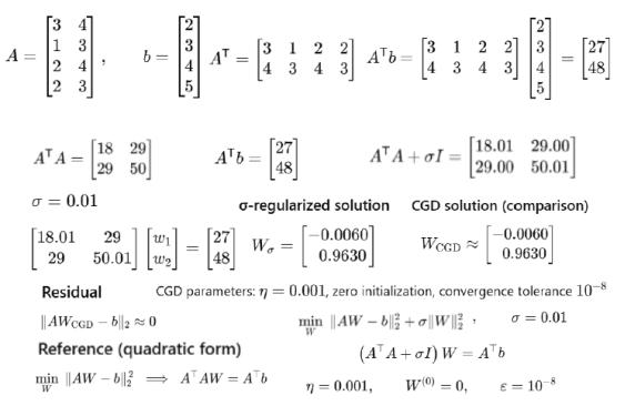
This solution is obtained in a single algebraic evaluation, without learning rates, initialization, stopping criteria, or iterative updates. In the numerical example reported in Figure 7, a small overdetermined system is solved using gradient descent (GD), conjugate gradient descent (CGD), and the σ-regularized deterministic method. All approaches converge to the same equilibrium vector W, as expected for a quadratic objective. However, their computational behavior differs substantially. Gradient descent requires a large number of iterations and careful parameter tuning, while conjugate gradient descent converges in fewer steps but still relies on iterative trajectory updates. In contrast, the Cekirge Method computes the equilibrium directly, in one step.

Despite the minimal size of the system, the runtime difference between iterative and closed-form solutions spans several orders of magnitude. This demonstrates that the inefficiency of iterative learning is structural rather than dimensional, arising from the formulation of learning as a trajectory rather than an equilibrium computation. Figure 7 defines the overdetermined test system, and illustrates the computation procedure and resulting closed-form equilibrium, demonstrating that even the simplest overdetermined learning problems do not require iterative optimization. Table 5 presents comparison of the Cekirge’s sigma method, GD and CGD. The Cekirge method naturally induces a mixture-of-experts–like structure when applied to clustered under- or overdetermined systems. Although conjugate gradient descent converges rapidly for very small systems, its iteration count and numerical stability degrade with dimension and conditioning, whereas the σ-regularized deterministic solution computes the same equilibrium in a single algebraic step independent of system size.

To provide an intuitive interpretation of equilibrium recognition versus iterative search, Table 6 summarizes the “Cekirge’s dog” metaphor used throughout this work.

Download: Download full-size image

Figure 7. The illustration of the mathematical analysis.

Table 5. Timing comparison.

Method	Iterations	Time scale	Time	Runtime Notes
GD	~50,000–100,000 ~70,000	10^-2 – 10^-1 s	ms–s	η sensitive Crawling toward equilibrium
CGD	2–3	10^-5 s	microseconds	Very fast, but still iterative
Cekirge (σ)	1	10^-8 s	microseconds	No iteration, Direct equilibrium

Table 6. The object John’s overdetermined system for the Cekirge’s dog.

Metaphor	Mathematics
John	Equilibrium solution W*
Ring / hat / jacket	Perturbations, noise, local variation
New pants	Different samples / batches
Dog recognition	σ-regularized equilibrium
Dog ignoring accessories	Stability under perturbation
Failing to recognize	GD chasing surface noise

For the overdetermined system, the σ-regularized normal operator yields a unique deterministic solution in closed-form, obtained in a single algebraic step without iterative optimization. A minimal overdetermined example highlights the structural inefficiency of iterative learning by contrasting gradient-based trajectories with the proposed one-shot σ-regularized equilibrium.

The normal operator A^TA is symmetric and positive semidefinite, but may be singular if the columns of A are linearly dependent; the addition of σ I guarantees strict positive definiteness and invertibility. Geometrically, A^TA defines the metric induced by the column geometry of A in parameter space and may exhibit flat directions when columns are linearly dependent. The addition of σ enforces uniform curvature in all directions, eliminating degeneracy and yielding a unique, stable equilibrium that can be computed directly. σ-regularization guarantees the existence and uniqueness of a solution, even when the unregularized normal system is singular or ill-conditioned.

1) Singularity is not a failure of algebra

2) It is a loss of identifiability

3) σ restores deterministic equilibrium

When the normal operator A^TA is singular or ill-conditioned, σ-regularization guarantees the existence of a unique solution by enforcing strict positive definiteness. As a result, learning is always well-posed and the equilibrium can be computed directly.

Normal Operator and σ-Regularization

The normal operator A^TA is symmetric and positive semidefinite, but it may be singular when the columns of A are linearly dependent. The addition of σI guarantees strict positive definiteness and invertibility, thereby restoring a unique and stable solution. Geometrically, A^TA defines the metric induced by the column geometry of A in parameter space. Linear dependence among columns introduces flat directions in the loss landscape. σ-regularization enforces uniform curvature in all directions, eliminating degeneracy and yielding a unique equilibrium that can be computed directly. σ-regularization therefore guarantees the existence and uniqueness of a well-posed solution, even when the unregularized normal system is singular or ill-conditioned.

Conceptual takeaway (Cekirge perspective)

1) Singularity is not a failure of algebra

2) It reflects a loss of identifiability

3) σ restores deterministic equilibrium

When the normal operator A^TA is singular or ill-conditioned, σ-regularization enforces strict positive definiteness, ensuring that learning remains well-posed and the equilibrium is obtained directly.

Recognition metaphor (dog intuition)

Just as a dog immediately recognizes its owner regardless of changes in clothing or accessories, the σ-regularized framework recognizes the equilibrium structure of the system without iterative search. Surface variations may change appearance, but identity remains intact; σ enables immediate recognition of that identity. The addition of σ guarantees a unique and stable equilibrium, enabling immediate recognition of the solution even in singular or overdetermined settings. The addition of σ guarantees a unique and stable solution even in singular or overdetermined settings.

1) “well-posed solution”

2) “unique solution”

3) “stable equilibrium”

Unified treatment of complete systems and conditioning

A linear system may be underdetermined, overdetermined, or fully determined; however, solvability alone does not guarantee numerical stability or reproducibility. Even for complete (square) systems, the coefficient matrix may be ill-conditioned or nearly singular, leading to sensitivity with respect to perturbations, measurement noise, or floating-point effects. Consequently, the distinction between well-conditioned and ill-conditioned systems is structurally more relevant than dimensionality alone.

For real-valued systems, left multiplication by the transpose yields the symmetric normal operator A^⊤A, which is positive semidefinite. In ill-conditioned or rank-deficient cases, this operator may lack invertibility or exhibit flat directions in parameter space. The addition of the σ-regularization term transforms the operator into A^⊤A + σ I, enforcing strict positive definiteness and guaranteeing existence, uniqueness, and numerical stability of the solution. This applies uniformly to underdetermined, overdetermined, and fully determined systems, regardless of conditioning.

Within the Cekirge framework, learning is therefore formulated as deterministic equilibrium recognition rather than iterative search. The σ-regularized equilibrium is computed directly in closed form, without reliance on iterative optimization, learning rates, or trajectory-based convergence. Conceptually, the Cekirge’s dog metaphor captures this unification: the equilibrium is recognized immediately and consistently, independent of surface variations such as system size, conditioning, or perturbations.

The Cekirge’s dog metaphor may be interpreted at the level of a biological neuron. Neural decision mechanisms do not perform long iterative searches; instead, they operate under severe energy constraints and converge rapidly to stable states. Biological systems minimize metabolic expenditure by settling into equilibrium configurations rather than executing prolonged update trajectories. While artificial optimization algorithms may rely on thousands of iterations, biological lifetimes and energy budgets are not sufficient for such repeated computations. Decision-making therefore favors immediate equilibrium recognition over iterative refinement, a principle reflected in the σ-regularized deterministic formulation, which computes the stable solution directly in a single step.

Biological decision systems effectively operate on ill-conditioned inputs, where surface variations-such as context, noise, or redundant features-act as σ-like perturbations; stability is achieved not by iteration, but by recognizing the underlying equilibrium despite these added degrees of freedom. These systems operate on inherently ill-conditioned inputs, where surface variations act as σ-like perturbations, yet stability is achieved through direct equilibrium recognition rather than iterative search.

Diagonal stabilization was first introduced analytically by Tikhonov to render ill-posed inverse problems well-posed. The same structure later appeared in statistics as ridge regression, formalized by Hoerl and Kennard. Subsequent work by Golub, Heath, and Wahba focused on selecting the regularization parameter through generalized cross-validation, reinforcing the view of regularization as a parameter-tuning process rather than an explicit equilibrium definition,

[11]

. Singularity is not a failure of algebra; it reflects a loss of identifiability. σ restores deterministic equilibrium. This perturbation-based interpretation of σ as a structural stabilizer is consistent with earlier analytical studies on conlinear system perturbations, where bounded equilibrium response under operator variations was explicitly characterized

[11]

8. Conclusion

The Cekirge Method demonstrates that σ-regularized learning is fundamentally an equilibrium computation, not an iterative optimization procedure. When the loss is quadratic and stabilized by σ, the stationary condition yields a unique and reproducible solution obtained in a single algebraic step. In contrast, gradient-based methods-GD, SGD, and CGD-depend on initialization, step size, sampling order, numerical precision, and stopping heuristics. Their trajectories traverse long update paths, whereas the σ-Method lands directly on the equilibrium.

This distinction is most clearly illustrated by Cekirge’s dog. A dog placed in a valley does not wander along the valley walls or descend by trial and error. It senses the geometric center of the basin-the intersection of the L₁ active faces and the curvature of the L₁ bowl-and settles at the minimum in one move, without iteration, drift, or uncertainty. The dog analogy captures the essence of deterministic learning:

Within this framework, equilibrium is recognized rather than searched for, and σ plays a fundamental analytical role. A^TA + σ I becomes strictly positive definite, guaranteeing existence, uniqueness, and stability of the equilibrium regardless of the conditioning of A^⊤A. Even an arbitrarily small σ removes ill-posedness entirely. The resulting solution is invariant across hardware platforms, floating-point precision, and computational architectures.

This restores the original mathematical purpose of Tikhonov regularization. Tikhonov introduced diagonal stabilization not as a penalty embedded within an iterative solver, but as an analytical correction that converts an ill-posed inverse problem into a well-posed one. With the rise of optimization-centric learning, this concept came to be interpreted through the lens of gradient descent. The Cekirge Method returns to the original meaning:

σ defines the equilibrium itself, not the target of an iterative search.

Once this analytical foundation is adopted, large-scale computation becomes straightforward. The deterministic σ-partition strategy decomposes the system into overlapping blocks, each solving its own σ-equilibrium. Overlaps transmit anchor energy between blocks-analogous to how biological systems integrate local sensory fields into a coherent global perception. By deterministically fusing these block equilibria, the method constructs a global solution without iteration, without tuning, and without numerical drift, extending σ-equilibrium computation far beyond the scale of a single matrix inversion.

The conclusion is unambiguous:

σ-regularization yields a unique, stable, and platform-independent equilibrium that does not rely on gradient descent or stochastic sampling. The Cekirge framework unifies classical inverse-problem theory, large-matrix computation, and biological principles of energetic balance into a single deterministic learning system.

In this formulation, learning is not a search- it is the algebraic realization of an equilibrium dictated by σ, recognized instantly, the way Cekirge’s dog finds the minimum without ever needing to descend into it.

Abbreviations

A	Data Matrix
A(k)	Local σ-Block Matrix
A_₀	Anchor Row (Unperturbed)
A^TA	Normal-Equation Matrix
b	Target Vector
b(k)	Prorated Block Target
bσ	σ-Perturbed Target Vector
C	System Matrix in the Energy Functional
CGD	Conjugate Gradient Descent
GD	Gradient Descent
SGD	Stochastic Gradient Descent
d	Feature Dimension
E(W)	Total σ-Regularized Energy
E(k)	Block σ-Energy
Eanchor(k)	Anchor Energy of Block k
k	Number of Overlapping σ-Blocks
L2(W)	Quadratic Loss Function
MAX(W)	Laplace (MAX) Loss Function
L_σ	Anchor-Loss for σ-Regularized Solution
N	Number of Samples
R(σ)	Relative Change in Anchor-Loss
σ	Stabilizing Regularization Parameter
σ-Method	Deterministic σ-Regularized Learning Method
σ-March	Sequential σ-Stability Evaluation Process
σ-Block	Overlapping Deterministic Block
σ-Equilibrium	Unique Stationary Point of the
σ-Regularized	System Sigma-regularized equilibrium
T	Target Vector in the Energy Formulation
W	Weight Vector
Wσ	σ-Regularized Deterministic Solution
W(k)	Local σ-Solution from Block k
W_global	Fused Global σ-Solution

Author Contributions

Huseyin Murat Cekirge is the sole author. The author read and approved the final manuscript.

Conflicts of Interest

The author declares no conflicts of interest.

References

[1]	Tikhonov, A. N. Solutions of Ill-Posed Problems. V. H. Winston & Sons, 1977.
[2]	Rumelhart, D. E., Hinton, G. E., & Williams, R. J. “Learning Representations by Back-Propagation of Errors.” Nature, 323(6088), 533–536, 1986. https://doi.org/10.1038/323533a0
[3]	Hinton, G. “Efficient Representations and Energy Constraints in Learning Systems.” AI Magazine, 45(1), 2024. https://doi.org/10.1609/aimag.v45i1.29517
[4]	Schmidhuber, J. “Deep Learning in Neural Networks: An Overview.” Neural Networks, 61, 85–117, 2015. https://doi.org/10.1016/j.neunet.2014.09.003
[5]	Friston, K. “The Free-Energy Principle in Cognition and AI.” Nature Neuroscience, 22(2), 2019. https://doi.org/10.1038/s41593-018-0310-6
[6]	Benton, R. “Spectral Stabilization and Regularization in Large Transformer Architectures.” arXiv: 2304.10211, 2023.
[7]	Zhuge, Y., Han, J., & Li, Z. “Spectral Regularization in Large-Scale Transformer Training for Energy-Efficient Convergence.” IEEE Transactions on Neural Networks and Learning Systems, 35(7), 8432–8447, 2024. https://doi.org/10.1109/TNNLS.2024.3321459
[8]	Lee, D., & Fischer, A. “Deterministic Matrix-Inversion Learning for Stable Transformer Layers.” Nature Machine Intelligence, 7(3), 215–228, 2025. https://doi.org/10.1038/s42256-025-00934-0
[9]	Patel, K., Ahmed, S., & Rana, P. “Low-Entropy Energy Models for Reproducible AI Systems: Toward Analytical Convergence.” Proceedings of the AAAI Conference on Artificial Intelligence, 39(1), 1021–1032, 2025. https://doi.org/10.1609/aaai.v39i1.30567
[10]	Nguyen, T., & Raginsky, M. “Scaling Laws and Deterministic Limits in High-Dimensional Learning Dynamics.” Journal of Machine Learning Research, 25(118), 1–32, 2024. http://jmlr.org/papers/v25/nguyen24a.html
[11]	Cekirge, H. M. “Tuning the Training of Neural Networks by Using the Perturbation Technique.” American Journal of Artificial Intelligence, 9(2), 107–109, 2025. https://doi.org/10.11648/j.ajai.20250902.11
[12]	Cekirge, H. M. “An Alternative Way of Determining Biases and Weights for the Training of Neural Networks.” American Journal of Artificial Intelligence, 9(2), 129–132, 2025. https://doi.org/10.11648/j.ajai.20250902.14
[13]	Cekirge, H. M. “Algebraic σ-Based (Cekirge) Model for Deterministic and Energy-Efficient Unsupervised Machine Learning.” American Journal of Artificial Intelligence, 9(2), 198–205, 2025. https://doi.org/10.11648/j.ajai.20250902.20
[14]	Cekirge, H. M. “Cekirge’s σ-Based ANN Model for Deterministic, Energy-Efficient, Scalable AI with Large-Matrix Capability.” American Journal of Artificial Intelligence, 9(2), 206–216, 2025. https://doi.org/10.11648/j.ajai.20250902.21
[15]	Cekirge, H. M. Cekirge_Perturbation_Report_v4. Zenodo, 2025. https://doi.org/10.5281/zenodo.17393651
[16]	Cekirge, H. M. “Algebraic Cekirge Method for Deterministic and Energy-Efficient Transformer Language Models.” American Journal of Artificial Intelligence, 9(2), 258–271, 2025. https://doi.org/10.11648/j.ajai.20250902.25
[17]	Cekirge, H. M. “Deterministic σ-Regularized Benchmarking of the Cekirge Model Against GPT-Transformer Baseline.” American Journal of Artificial Intelligence, 9(2), 272–280, 2025. https://doi.org/10.11648/j.ajai.20250902.26
[18]	Cekirge, H. M. “The Cekirge Method for Machine Learning: A Deterministic σ-Regularized Analytical Solution for General Minimum Problems.” American Journal of Artificial Intelligence, 9(2), 324–337, 2025. https://doi.org/10.11648/j.ajai.20250902.31
[19]	Golub, G. H., Heath, M., & Wahba, G., “Generalized Cross-Validation as a Method for Choosing a Good Ridge Parameter.”Technometrics, 21(2), 215–223, 1979.
[20]	Hoerl, A. E., & Kennard, R. W., “Ridge Regression: Biased Estimation for Nonorthogonal Problems.” Technometrics, 12(1), 55–67, 1970.

Cite This Article

Plain Text BibTeX RIS

APA Style

Cekirge, H. M. (2026). The Cekirge σ-Method in AI: Analysis and Broad Applications. American Journal of Artificial Intelligence, 10(1), 14-33. https://doi.org/10.11648/j.ajai.20261001.12

Copy | Download

ACS Style

Cekirge, H. M. The Cekirge σ-Method in AI: Analysis and Broad Applications. Am. J. Artif. Intell. 2026, 10(1), 14-33. doi: 10.11648/j.ajai.20261001.12

Copy | Download

AMA Style

Cekirge HM. The Cekirge σ-Method in AI: Analysis and Broad Applications. Am J Artif Intell. 2026;10(1):14-33. doi: 10.11648/j.ajai.20261001.12

Copy | Download

@article{10.11648/j.ajai.20261001.12,
  author = {Huseyin Murat Cekirge},
  title = {The Cekirge σ-Method in AI: Analysis and Broad Applications},
  journal = {American Journal of Artificial Intelligence},
  volume = {10},
  number = {1},
  pages = {14-33},
  doi = {10.11648/j.ajai.20261001.12},
  url = {https://doi.org/10.11648/j.ajai.20261001.12},
  eprint = {https://article.sciencepublishinggroup.com/pdf/10.11648.j.ajai.20261001.12},
  abstract = {Modern machine learning relies predominantly on iterative optimization, assuming that learning must progress by following gradients across a probabilistic loss landscape shaped by Gaussian noise. Such methods depend on learning rates, random initialization, batching strategies, and repeated parameter updates, and their outcomes vary with numerical precision, hardware behavior, and floating-point drift. As dimensionality increases or data matrices become ill-conditioned, these iterative procedures often require extensive tuning and may converge inconsistently or fail altogether. This work presents the Cekirge Global Deterministic σ-Method, a non-iterative learning framework in which model parameters are obtained through a single closed-form computation rather than through iterative descent. Learning is formulated as a deterministic equilibrium problem governed by a σ-regularized equilibrium functional. A behavioral analogy-Cekirge’s Dog-illustrates the operational distinction: a trained working dog runs directly to its target without scanning or correcting its path step by step, whereas iterative algorithms resemble a dog that repeatedly stops, senses, and adjusts direction. Throughout this work, the term equilibrium functional is used instead of energy, emphasizing deterministic balance rather than physical or variational interpretations. The proposed framework yields a unique, reproducible solution independent of initialization or hardware, remains stable for ill-conditioned systems, and scales deterministically to large problems through σ-regularized partitioning. A minimal overdetermined example demonstrates that the inefficiency of gradient-based learning is structural rather than dimensional, arising from trajectory-based optimization, while the proposed σ-regularized formulation computes the same equilibrium directly in a single closed-form step.},
 year = {2026}
}

Copy | Download

TY  - JOUR
T1  - The Cekirge σ-Method in AI: Analysis and Broad Applications
AU  - Huseyin Murat Cekirge
Y1  - 2026/01/19
PY  - 2026
N1  - https://doi.org/10.11648/j.ajai.20261001.12
DO  - 10.11648/j.ajai.20261001.12
T2  - American Journal of Artificial Intelligence
JF  - American Journal of Artificial Intelligence
JO  - American Journal of Artificial Intelligence
SP  - 14
EP  - 33
PB  - Science Publishing Group
SN  - 2639-9733
UR  - https://doi.org/10.11648/j.ajai.20261001.12
AB  - Modern machine learning relies predominantly on iterative optimization, assuming that learning must progress by following gradients across a probabilistic loss landscape shaped by Gaussian noise. Such methods depend on learning rates, random initialization, batching strategies, and repeated parameter updates, and their outcomes vary with numerical precision, hardware behavior, and floating-point drift. As dimensionality increases or data matrices become ill-conditioned, these iterative procedures often require extensive tuning and may converge inconsistently or fail altogether. This work presents the Cekirge Global Deterministic σ-Method, a non-iterative learning framework in which model parameters are obtained through a single closed-form computation rather than through iterative descent. Learning is formulated as a deterministic equilibrium problem governed by a σ-regularized equilibrium functional. A behavioral analogy-Cekirge’s Dog-illustrates the operational distinction: a trained working dog runs directly to its target without scanning or correcting its path step by step, whereas iterative algorithms resemble a dog that repeatedly stops, senses, and adjusts direction. Throughout this work, the term equilibrium functional is used instead of energy, emphasizing deterministic balance rather than physical or variational interpretations. The proposed framework yields a unique, reproducible solution independent of initialization or hardware, remains stable for ill-conditioned systems, and scales deterministically to large problems through σ-regularized partitioning. A minimal overdetermined example demonstrates that the inefficiency of gradient-based learning is structural rather than dimensional, arising from trajectory-based optimization, while the proposed σ-regularized formulation computes the same equilibrium directly in a single closed-form step.
VL  - 10
IS  - 1
ER  -

Copy | Download

Author Information

Huseyin Murat Cekirge

Department of Mechanical Engineering, The City College of New York (CUNY), New York, USA

Contact Email

http://orcid.org/0000-0001-8075-2306

Download PDF

Submit an Article

Figure 1

Figure 1. Geometric equivalence of L₁ and L₂ minima under σ-regularized deterministic equilibrium.
Figure 2

Figure 2. Illustrates the test matrix considered.
Figure 3

Figure 3. Blocks of a large matrix.
Figure 4

Figure 4. Blocks of a large matrix.
Figure 5

Figure 5. The first block.
Figure 6

Figure 6. The second Block.
Figure 7

Figure 7. The illustration of the mathematical analysis.

Table 1

Table 1. Deterministic σ-Equilibrium Solutions for an 8×8 Anchor-Repeat System (b = 5).
Table 2

Table 2. Deterministic σ-Equilibrium Solutions for an 8×8 Anchor-Repeat System under Target Perturbation (b = (5+σ)·1).
Table 3

Table 3. The partition calculation for σ =0.01.
Table 4

Table 4. The partition calculation for σ =0.1.
Table 5

Table 5. Timing comparison.
Table 6

Table 6. The object John’s overdetermined system for the Cekirge’s dog.

Plain Text BibTeX RIS

APA Style

Cekirge, H. M. (2026). The Cekirge σ-Method in AI: Analysis and Broad Applications. American Journal of Artificial Intelligence, 10(1), 14-33. https://doi.org/10.11648/j.ajai.20261001.12

Copy | Download

ACS Style

Cekirge, H. M. The Cekirge σ-Method in AI: Analysis and Broad Applications. Am. J. Artif. Intell. 2026, 10(1), 14-33. doi: 10.11648/j.ajai.20261001.12

Copy | Download

AMA Style

Cekirge HM. The Cekirge σ-Method in AI: Analysis and Broad Applications. Am J Artif Intell. 2026;10(1):14-33. doi: 10.11648/j.ajai.20261001.12

Copy | Download

@article{10.11648/j.ajai.20261001.12,
  author = {Huseyin Murat Cekirge},
  title = {The Cekirge σ-Method in AI: Analysis and Broad Applications},
  journal = {American Journal of Artificial Intelligence},
  volume = {10},
  number = {1},
  pages = {14-33},
  doi = {10.11648/j.ajai.20261001.12},
  url = {https://doi.org/10.11648/j.ajai.20261001.12},
  eprint = {https://article.sciencepublishinggroup.com/pdf/10.11648.j.ajai.20261001.12},
  abstract = {Modern machine learning relies predominantly on iterative optimization, assuming that learning must progress by following gradients across a probabilistic loss landscape shaped by Gaussian noise. Such methods depend on learning rates, random initialization, batching strategies, and repeated parameter updates, and their outcomes vary with numerical precision, hardware behavior, and floating-point drift. As dimensionality increases or data matrices become ill-conditioned, these iterative procedures often require extensive tuning and may converge inconsistently or fail altogether. This work presents the Cekirge Global Deterministic σ-Method, a non-iterative learning framework in which model parameters are obtained through a single closed-form computation rather than through iterative descent. Learning is formulated as a deterministic equilibrium problem governed by a σ-regularized equilibrium functional. A behavioral analogy-Cekirge’s Dog-illustrates the operational distinction: a trained working dog runs directly to its target without scanning or correcting its path step by step, whereas iterative algorithms resemble a dog that repeatedly stops, senses, and adjusts direction. Throughout this work, the term equilibrium functional is used instead of energy, emphasizing deterministic balance rather than physical or variational interpretations. The proposed framework yields a unique, reproducible solution independent of initialization or hardware, remains stable for ill-conditioned systems, and scales deterministically to large problems through σ-regularized partitioning. A minimal overdetermined example demonstrates that the inefficiency of gradient-based learning is structural rather than dimensional, arising from trajectory-based optimization, while the proposed σ-regularized formulation computes the same equilibrium directly in a single closed-form step.},
 year = {2026}
}

Copy | Download

TY  - JOUR
T1  - The Cekirge σ-Method in AI: Analysis and Broad Applications
AU  - Huseyin Murat Cekirge
Y1  - 2026/01/19
PY  - 2026
N1  - https://doi.org/10.11648/j.ajai.20261001.12
DO  - 10.11648/j.ajai.20261001.12
T2  - American Journal of Artificial Intelligence
JF  - American Journal of Artificial Intelligence
JO  - American Journal of Artificial Intelligence
SP  - 14
EP  - 33
PB  - Science Publishing Group
SN  - 2639-9733
UR  - https://doi.org/10.11648/j.ajai.20261001.12
AB  - Modern machine learning relies predominantly on iterative optimization, assuming that learning must progress by following gradients across a probabilistic loss landscape shaped by Gaussian noise. Such methods depend on learning rates, random initialization, batching strategies, and repeated parameter updates, and their outcomes vary with numerical precision, hardware behavior, and floating-point drift. As dimensionality increases or data matrices become ill-conditioned, these iterative procedures often require extensive tuning and may converge inconsistently or fail altogether. This work presents the Cekirge Global Deterministic σ-Method, a non-iterative learning framework in which model parameters are obtained through a single closed-form computation rather than through iterative descent. Learning is formulated as a deterministic equilibrium problem governed by a σ-regularized equilibrium functional. A behavioral analogy-Cekirge’s Dog-illustrates the operational distinction: a trained working dog runs directly to its target without scanning or correcting its path step by step, whereas iterative algorithms resemble a dog that repeatedly stops, senses, and adjusts direction. Throughout this work, the term equilibrium functional is used instead of energy, emphasizing deterministic balance rather than physical or variational interpretations. The proposed framework yields a unique, reproducible solution independent of initialization or hardware, remains stable for ill-conditioned systems, and scales deterministically to large problems through σ-regularized partitioning. A minimal overdetermined example demonstrates that the inefficiency of gradient-based learning is structural rather than dimensional, arising from trajectory-based optimization, while the proposed σ-regularized formulation computes the same equilibrium directly in a single closed-form step.
VL  - 10
IS  - 1
ER  -

Copy | Download