Successive Regression to Determine the Optimum Terrain Correction Density in Mountainous Areas

Gao Weiqiang; Shi Zhaoyang; Zhang Liming; Feng Xuliang

doi:doi:10.11648/j.earth.20251404.13

Research Article |

| Peer-Reviewed

Successive Regression to Determine the Optimum Terrain Correction Density in Mountainous Areas

Gao Weiqiang

, Shi Zhaoyang

, Zhang Liming

, Feng Xuliang^*

Published in Earth Sciences (Volume 14, Issue 4)

Received: 2 July 2025 Accepted: 18 July 2025 Published: 13 August 2025

Views: Downloads:

Download PDF

Share This Article

Twitter
Linked In
Facebook

Abstract

Bouguer gravity anomalies are generally correlated with topography in mountainous regions. However, their applicability in geological interpretations of gravity data is often constrained by inaccuracies in terrain correction density. To address this limitation, this study employed regression analysis to ascertain the most suitable terrain correction density by investigating the interplay between free-air gravity anomalies and elevation. The density values were then iteratively refined based on the dynamic relationship between computed Bouguer gravity anomalies and elevation at each stage of iteration. By continuously adjusting the terrain correction density throughout the topographic correction process, we ultimately determined the optimal density value and its corresponding Bouguer gravity anomaly. This methodology was applied to gravity data gathered from Jiuzong Mountain, where the ideal terrain correction density was attained after five iterative cycles. The resultant Bouguer gravity anomaly was subsequently calculated, and the efficacy of the proposed method was corroborated by the empirical findings derived from Jiuzhong Mountain.

Published in	Earth Sciences (Volume 14, Issue 4)
DOI	10.11648/j.earth.20251404.13
Page(s)	149-159
Creative Commons	This is an Open Access article, distributed under the terms of the Creative Commons Attribution 4.0 International License (http://creativecommons.org/licenses/by/4.0/), which permits unrestricted use, distribution and reproduction in any medium or format, provided the original work is properly cited.
Copyright	Copyright © The Author(s), 2025. Published by Science Publishing Group

Keywords

Bouguer Gravity Anomaly, Iterative Regression, Jiuzong Mountain, Terrain Correction, Density Optimization

1. Introduction

After applying height, latitude, terrain, and intermediate layer corrections to measured gravity data, the Bouguer gravity anomaly can be obtained. This anomaly serves as the foundation for interpreting gravity data. However, in mountainous regions characterized by significant variations in terrain, Bouguer gravity anomalies often exhibit strong correlations with changes in terrain elevation, which is a phenomenon referred to as mountain-shaped anomalies

[1, 2]

. These anomalies present considerable challenges to the interpretation and inference of geological structures.

The primary cause of abnormal gravity anomalies in mountainous regions is inaccuracies in determining the density of the intermediate layer during topographic corrections

[3]

. The density of the middle layer can be inversely calculated using the intermediate layer correction coefficient, C = 2πGσ, which is obtained by fitting the measured gravity data with the elevation scatter plot

[2, 4]

. However, in mountainous areas with significant topographic undulations, the scale of the topographic material is reduced, and the resulting gravity effect is smaller than the gravity effect of the Bouguer plate, which leads to an underestimation of the calculated middle layer density

[1]

. Thorarinsson and Magnusson pioneered the use of fractal analysis in the field of gravity exploration and achieved good geological results in southwestern Iceland

[5]

. However, this technique involves dividing the complex surface into zones that have the same density layer, and the more uniform the rock density within the zone is, the better the method works

[6]

. Therefore, this method is difficult to apply in practice

[7]

The correlation analysis method represents a conventional approach for determining the optimal intermediate layer density. Typically, a series of intermediate layer density values are applied to correct the gravity profile; the density corresponding to the Bouguer gravity anomaly that exhibits minimal correlation with topography is selected as the optimal intermediate layer density

[8, 9]

. Within the same survey area, if the surface density is relatively homogeneous, the graphical profile method is effective

[10]

. Conversely, the density derived from the graphical method pertains solely to the specific profile location and does not adequately represent the density distribution across the entire survey area

[10, 11]

. A correlation analysis can be performed between the post density correction Bouguer gravity anomaly and terrain elevation for the entire region, and the density with the least correlation is selected as the optimal value for density correction

[11]

. In cases where the lateral surface density varies significantly, the optimal density values can be determined on a zonal basis and subsequently integrated to form a spatially varying intermediate layer density model for the entire area

[12]

. Alternatively, compensation corrections may be applied on the basis of results of constant-density corrections

[13-15]

. However, when dealing with large study areas requiring zonal calculations, the computational burden becomes substantial, and the resulting density values approximate but do not necessarily reflect the most "accurate" intermediate layer density.

Cai Shangzhong established the functional relationship between free-space gravity anomalies and elevation

[2]

. The regression anomaly was subsequently computed on the basis of the actual elevation of each measurement point and removed from the measured free-space gravity anomaly to derive the regression residual anomaly, which facilitates qualitative interpretation. For large study areas, the sliding window regression analysis method can be employed, with the variogram providing a quantitative reference for selecting the window size

[16]

. However, only the relationship between terrain and gravity anomalies within the study area is accounted for in the regression analysis method. The resulting gravity values obtained via regression analysis represent only those anomalies that exhibit overall regional variations correlated with terrain undulations. This method cannot eliminate local anomalies, particularly those influenced by terrain outside the study area. Furthermore, the regional anomalies removed by this method may include useful gravity anomalies associated with deep geological structures.

If the measured rock densities from surface geological outcrops in the study area are available, interpolation and smoothing techniques can be utilized to construct a surface density distribution model. Furthermore, a floating datum plane can be established for terrain and intermediate layer corrections

[7]

. However, when the study area is extensive, the limited sampling of outcrops and borehole measurements may not fully capture the variations in surface rock density across the survey region. To address this limitation, Niu Yuanyuan et al. developed an approach based on one-dimensional free-air gravity anomaly data and employed Bayesian methods to estimate near-surface rock densities

[17]

. The estimated densities are highly consistent with surface geological characteristics and regional stratigraphic density data. Nonetheless, this method has thus far been applied only to profile gravity anomaly analyses, with no reported applications to areal gravity anomalies.

Gravity data inherently contain information regarding both structural and density characteristics. Previous studies have demonstrated the feasibility of accurately estimating near-surface rock densities or density contrasts across density interfaces using gravity data

[17, 18]

. Florio

[19, 20]

employed regression analysis to invert the depth of sedimentary basin basement and estimate the density contrast between the sedimentary layer and the basement. The Bayesian estimation method requires the application of cubic spline fitting to model gravity profile variations, which can be extended to areal gravity inversion. However, cubic spline surface fitting entails a large number of computational parameters and imposes a significant computational burden. The ITerative RESCaling method (ITRESC) method introduced by Florio utilizes geophysical well logging or other geophysical data to provide depth constraints and construct depth-gravity value models; however, it does not adequately account for lateral variations within sedimentary basins and their basement structures. Drawing upon these methodologies, this study applied the Bouguer plate calculation formula in conjunction with successive regression techniques to analyze optimal density corrections. The proposed approach was implemented for external correction of gravity data in the Jiuzong Mountain region of Zhao Mausoleum, integrating high-precision gravity data with practical considerations, thereby achieving both computational efficiency and favorable application results.

2. Results

2.1. Overview of the Study Area

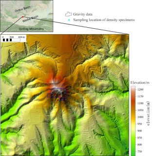
Jiuzong Mountain is located on the southern margin of the Ordos Basin; this mountain is adjacent to the Qilian-Hexi Corridor (Liupan Mountain)-Helan Mountain tectonic belt to the west and is separated from the Qinling Orogenic Belt by the Wei River Basin to the south. This mountain lies between the stable Ordos Block and the active Qilian-Qinling Orogenic Belt (Figure 1), which has a long, complex geological tectonic history. The study area is situated in the inverted structural zone along the southern margin of the Ordos Basin and is characterized as a strong near-east west-trending folding zone. The overall structural form is a complex anticline, with secondary anticlines and synclines distributed in a band-like pattern from east to west. These structures feature tight folds, local southward inversion, and frequent faults on both flanks. The core of the royal tombs of the Tang dynasty syncline comprises the upper Ordovician the royal tombs of the Tang dynasty formation. The southern limb dips northward at 350°-10°∠20°-30°, whereas the northern limb dips southward with a steeper inclination. The general dip direction is 170°-190°∠50°-60°. Owing to the disruption caused by the north-dipping fault on the northern limb, the stratigraphic sequence is incompletely exposed, which results in an asymmetric syncline structure.

Download: Download full-size image

Figure 1. The topographic map obtained by the UAV LiDAR survey of Jiuzong Mountain and its adjacent area.

The study area is located on the southern limb of the royal tombs of the Tang dynasty Mausoleum syncline. The exposed Ordovician royal tombs of the Tang dynasty Mausoleum Formation can be stratigraphically divided into two distinct lithological units. The lower unit (O₃t₁) consists of various (yellowish-brown, grayish-green, purplish-red, and dark gray) gravelly shales. At its base, thick-bedded lithic sandstones are intercalated and large boulders of dolomite with chert bands occur. The upper unit (O₃t₂) consists of gray and light gray extremely thick-bedded polymict conglomerates and breccias, with occasional intercalations of gravelly sandstones. The contact between the lower and upper units is conformable.

2.2. Geophysical Characteristics

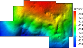
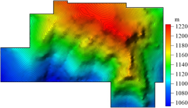
A total of 1,722 gravity measurement points were acquired in the study area, with a line spacing of 10m and a point spacing of 5 m. The original gravity data were corrected for elevation and normal field effects, and the free-air gravity anomaly is depicted in Figure 2. This anomaly has a distinct covarying relationship with topography (Figure 3). Within an altitude variation range of less than 200 m, the local variations in the gravity anomaly approach 10×10^-5 m/s².

Download: Download full-size image

Figure 2. Free-air gravity anomalies in the study area.Free-air gravity anomalies in the study area.

Table 1. Statistics on the density of various rocks in the researched area.

Lithology	Number	Range of density variation/×10³kg/m³	Average density/×10³kg/m³
Arenite siltstone	15	2.574~2.815	2.676
Polemic conglomerate	9	2.637~2.783	2.704
Conglomerate	74	2.404~2.812	2.734
Sandy conglomerate	8	2.706~2.820	2.773
Variegatedmud-bearing sandy conglomerate	9	2.559~2.714	2.659
Motley conglomerate	7	2.749~2.812	2.771
Vermilion conglomerate	8	2.608~2.772	2.700
Marble (Zhuoshan Jade)	6	2.635~2.667	2.655
Quartzitic sandstone	2		2.775
Grey mud-bearing sandy conglomerate	2		2.457
Grey thick-bedded polymict conglomerate	3		2.777
Dolomite	2		2.788
Calcareous rock	2		2.725
Argillaceous siltstone	3		2.648
Argillaceous arenaceous conglomerate	2		2.631
Arenaceous shale	1		2.727
Tang Dynasty tile	2		1.792
Bricks from the Tang Dynasty	1		2.214

The study area is characterized predominantly by extensive exposure of the Ordovician the royal tombs of the Tang dynasty mausoleum formation. The Quaternary strata are notably thin and distributed only in localized areas with a maximum thickness not exceeding 1 m. Given the absence of terrain correction density data for the study area, the densities of 156 rock samples were measured at various locations (as indicated by the blue stars in Figure 1). The statistical results are presented in Table 1. Overall, the rocks within the study area exhibit relatively high densities, with most values clustering at approximately 2.7×10³kg/m³. Notably, the densities of glutenite and variegated conglomerate exceed 2.77×10³kg/m³. Despite the predominant exposure of the Ordovician the royal tombs of the Tang dynasty mausoleum formation, significant lithological heterogeneities within the formation clearly result in nonuniform density distributions, which exhibit distinct local variations.

Download: Download full-size image

Figure 3. The topography in the research area.The topography in the research area.

2.3. Results of Conventional Topographic Correction

Yan Liangjun et al. constructed lateral density variations on the basis of measured surface density data and applied them to topographic corrections, which yielded favorable geological outcomes

[7]

. In this study, the rock density values measured at 153 points (excluding those corresponding to Tang tiles and Tang bricks) were gridded to establish a variable-density model of the surface layer for topographic correction purposes. To prevent distortions in the Bouguer gravity anomaly caused by density discontinuities, the original density grid data were smoothed. Furthermore, when surface geological data were leveraged, the rock densities beyond the measured area were inferred, supplemented, and extended. Lateral variable-density data that were consistent with the topographic extent depicted in Figure 1 were ultimately obtained and utilized as the foundation for topographic corrections.

The Bouguer gravity anomaly can be derived by applying a topographic correction and an intermediate-layer correction to the free-air gravity anomaly. Traditionally, the terrain surrounding any measurement point is first "leveled and filled;" the gravitational effect of an infinitely large material layer between each measurement point and the base point is then calculated using the Bouguer plate formula. This calculation involves applying a topographic correction prior to the intermediate-layer correction. When determining the topographic correction value for a measurement point, the topographic correction values of four adjacent nodes near the measurement point are initially calculated, and then these values are interpolated to the measurement point's location to represent its topographic correction value

[21]

In this study, during the topographic correction process, the gravitational variations caused by the terrain at each gravity measurement point within the study area were computed directly on the basis of the measured topographic undulations. These variations were subsequently subtracted from the free-air gravity values to obtain the Bouguer gravity anomaly. This approach is used to effectively integrate traditional topographic and intermediate-layer corrections into a single step, simplifying the calculation procedure and eliminating interpolation errors associated with topographic correction values. Consequently, unless otherwise stated, the term "topographic correction" in this paper encompasses both traditional topographic and intermediate-layer corrections.

If gravity measurements are exclusively utilized for investigating local anomalies within a relatively small study area, topographic corrections can be performed within a maximum radius of 20km. The topographic correction for distant areas can be treated as a regional anomaly and eliminated

[22]

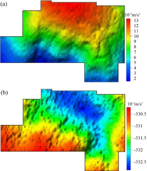
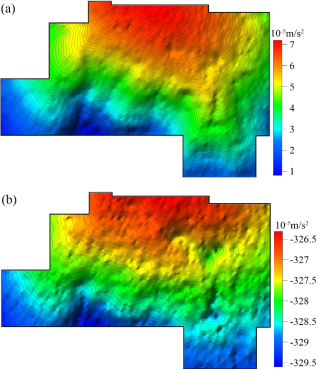
. The primary objective of the gravity survey in the Jiuzong Mountain study area was to deduce the location of the Zhao Mausoleum passage and the structure of the tomb chamber, which represents local shallow-surface target bodies. Consequently, in this study, only the influence of terrain within the range depicted in Figure 1 is quantified; the effects of terrain outside this region are neglected. To calculate the influence of the terrain, the position of the lowest measurement point was designated the base point. Additionally, the overall trend of terrain variations beyond the measurement points was considered. Ultimately, an elevation of 1000m was selected as the reference plane for the base point. Forward modeling was employed to compute the gravity anomalies induced by the material between the measured terrain surface and this reference plane at each measurement point, as illustrated in Figure 4a. By subtracting the terrain-induced effects from the free-air gravity anomalies, the Bouguer gravity anomalies were derived, as shown in Figure 4b.

Download: Download full-size image

Figure 4. The gravity effects caused by terrain are calculated using the actual density and the corresponding Bouguer gravity anomaly. (a) Gravity effects caused by terrain. (b) The Bouguer gravity anomaly.The gravity effects caused by terrain are calculated using the actual density and the corresponding Bouguer gravity anomaly. (a) Gravity effects caused by terrain. (b) The Bouguer gravity anomaly.

The Bouguer gravity anomaly depicted in Figure 4b has a mirror-image relationship with the terrain and is characterized by a pronounced mountain-shaped anomaly. The Bouguer gravity anomaly and topographic data prior to correction were normalized, resulting in a correlation coefficient of -0.989 between the two datasets, which indicates that the Bouguer gravity anomaly is substantially influenced by the terrain. As shown in Figure 4a, the variation pattern of the terrain influence closely mirrors that of the free-air gravity anomaly, with a correlation coefficient of 0.996. However, the relative variation of the former is significantly greater than that of the latter. This discrepancy arises because the terrain correction density derived from the measured data is overestimated. Field investigations revealed that the surface rocks in the study area are severely weathered resulting in an actual equivalent density that is much lower than the measured density. 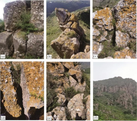Figure 5 presents photographs of surface rock outcrops at various measurement points. Specifically, Figure 5a-5e provide top-down views of the measurement points, whereas Figure 5f offers a long-distance view of the study area. Observations indicate that rock fractures are highly developed, with substantial variations in fracture scale across different locations and significant vertical extensions. Moreover, certain fractures are filled with loess, whereas others remain unfilled. The variability in fracture scales and fillings within the study area renders it impractical to estimate the optimal terrain correction density based solely on the measured rock density and fracture development degree. Consequently, an indirect method must be employed, which involves estimating the terrain correction density on the basis of the relationship between the actual terrain and the gravity anomaly.

Download: Download full-size image

Figure 5. Photographs of outcrops at several gravity measurement points.Photographs of outcrops at several gravity measurement points.

2.4. Method and Application of Successive Regression for Selecting the Terrain Correction Density

In mountainous regions with significant terrain undulations, the terrain correction density derived from the Bouguer plate formula is often underestimated when measured gravity data and elevation scatter plots are used to fit the intermediate layer correction coefficient

[1]

. This density can be iteratively adjusted to achieve the optimal terrain correction density. When inverting the depth of the density interface using gravity data, the Bouguer plate gravity formula is typically employed to construct an iterative calculation formula for the modification amount of the density interface depth. Through successive iterations, residual gravity anomaly values can be eliminated to obtain the depth of the density interface

[23, 24]

. Based on this iterative method, in this study, the following steps are adopted to determine the optimal terrain correction density:

Step 1: On the basis of the scatter plot of free-air gravity anomalies versus elevation, a fitting process is conducted using appropriate formulas to calculate the initial terrain correction density

σ_{(1)} = a / (1.6 πG)

. Here, G denotes the gravitational constant. Importantly, under three-dimensional conditions, the gravity change induced by the actual terrain is smaller in magnitude than the gravity anomaly of a Bouguer plate with the same density. Consequently, in this study, the coefficient in the Bouguer plate formula is adjusted to accelerate the iterative convergence process (changing

2 πG

to 1.6πG).

Step 2: Define

σ_{(1)}

as the terrain correction density. A forward-modeling computation is performed to determine the gravitational influence value

{g_{t}}_{(1)}

of the terrain at the measurement points. The Bouguer gravity anomaly is subsequently calculated using the formula (

g_{B (1)} = g_{f} - {g_{t}}_{(1)}

). A scatter plot of the free-air gravity anomaly versus the first-calculated gravitational influence value of the terrain at the measurement points was used to conduct a fitting analysis using the formula (

g_{f} = c \cdot g_{t (1)} + d

). The coefficient c is evaluated as follows: if c is significantly greater than 1, then the calculated gravitational influence value of the terrain is underestimated, and the terrain correction density is also underestimated. Then, if c is significantly less than 1, the calculated gravitational influence value of the terrain is overestimated, and the terrain correction density

σ_{(1)}

is also overestimated; proceed to the next step. If c is approximately 1, then this suggests that the terrain correction density

σ_{(1)}

is appropriately determined. At this point, the iteration process is terminated, and the Bouguer gravity anomaly is adopted as the final result.

On the basis of the scatter plot of the Bouguer gravity anomaly derived from the initial calculation and the corresponding elevation data, a fitting analysis was conducted using the formula (

g_{B (1)} = e \cdot h + f

). The first adjustment value for the terrain correction density is subsequently computed as (

δ σ_{(1)} = e / (1.6 πG)

Step 4: Based on formula (

σ_{(2)} = σ_{(1)} + δ σ_{(1)}

), the second terrain correction density is computed. Subsequently, set (

σ_{(1)} = σ_{(2)}

) and revert to Step 2 for further iterations.

Download: Download full-size image

Figure 6. Scatter points show the relationship between the free-air gravity anomaly and elevation in the research area.Scatter points show the relationship between the free-air gravity anomaly and elevation in the research area.

Download: Download full-size image

Figure 7. The gravity effects caused by terrain are calculated using the first regressed density and the corresponding Bouguer gravity anomaly. (a) Gravity effects caused by terrain. (b) The Bouguer gravity anomaly.The gravity effects caused by terrain are calculated using the first regressed density and the corresponding Bouguer gravity anomaly. (a) Gravity effects caused by terrain. (b) The Bouguer gravity anomaly.

Download: Download full-size image

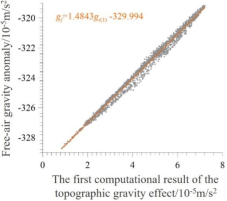
Figure 8. Scatter points show the relationship between the free-air gravity anomaly and gravity anomaly caused by terrain in the research area.Scatter points show the relationship between the free-air gravity anomaly and gravity anomaly caused by terrain in the research area.

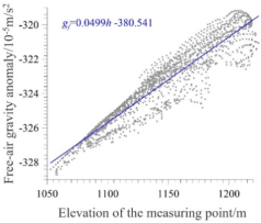
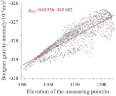
Following the aforementioned steps, the Bouguer gravity anomaly in the Jiuzong Mountain region is calculated in this study. A scatter plot of the free-air gravity anomaly versus the measurement point elevation, along with the fitting formula, is presented in Figure 6. The first terrain correction density value (

σ_{(1)} = 1.489

×10³kg/m³) is derived from the coefficient of the first-order term of the fitted model. On this basis, the terrain-induced gravity effect and the corresponding Bouguer gravity anomaly are computed, as illustrated in Figure 7a and 7b. At this stage, the scatter plot (Figure 8) of the free-air gravity anomaly against the terrain effect shown in Figure 7a reveals that the coefficient of the first-order term of the linear fit is 1.4843, which is significantly greater than 1. This indicates that the calculated terrain effect value is underestimated. According to the scatter plot of the Bouguer gravity anomaly versus elevation (Figure 9), the correction value for the first terrain correction (

δ σ_{(1)} = 0.463

×10³kg/m³) is obtained from the coefficient of the first-order term of the fitted model. Consequently, the second terrain correction density is determined to be (

σ_{(2)} = 1.952

×10³kg/m³).

Download: Download full-size image

Figure 9. Scatter points show the relationship between the first calculated Bouguer gravity anomaly and elevation in the research area.Scatter points show the relationship between the first calculated Bouguer gravity anomaly and elevation in the research area.

Download: Download full-size image

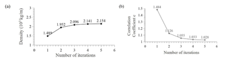
Figure 10. Variation in the density and correlation coefficient with an increasing number of iterations. (a) Density. (b) The correlation coefficient between the free-air gravity anomaly and gravity anomaly caused by terrain. Variation in the density and correlation coefficient with an increasing number of iterations. (a) Density. (b) The correlation coefficient between the free-air gravity anomaly and gravity anomaly caused by terrain.

By using this method, the optimal terrain correction density (

σ_{(5)} = 2.154

×10³ kg/m³) was determined after five iterations. The variation in the terrain correction density with respect to the number of iterations is illustrated in Figure 10a. The change in the correlation coefficient c, which represents the relationship between the free-air gravity anomaly and the calculated gravitational effect of the terrain at the measurement points as a function of the number of iterations, is depicted in Figure 10b. During the early stages of iteration, the density significantly varies with the number of iterations. As the number of iterations increases, the changes in density become less pronounced, and the correlation coefficient c gradually approaches 1. This suggests that the optimal density has been achieved at this point, and increasing the number of iterations provides minimal additional benefit. Assuming that the average density of surface rocks in the study area is 2.7×103, the optimal density value corresponds to approximately 80% of the density of unweathered rocks. On the basis of observations of fissure development in the exposed surface rocks, the estimated degree of fissure development ranges from 10% to 30%. Considering that partial loess fills the fissures, the optimal terrain correction density estimated in this study is reasonable. 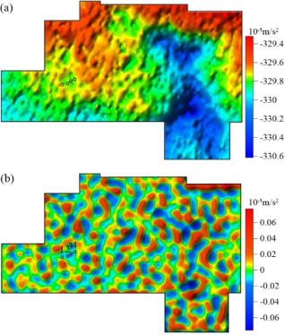The Bouguer gravity anomaly calculated using this density is presented in Figure 11a. Its correlation coefficient with the terrain is only 0.0329, which indicates that the Bouguer gravity anomaly is effectively independent of the terrain.

In the study area, four stone caves of varying sizes exist (their locations are indicated by the black boxes in Figure 11). Each cave has dimensions that are approximately 4m (width) × 3m (height) × 5.5m (depth), and the top of each stone cave is located approximately 8-10 m below the ground surface. If the average density of the intermediate layer estimated above is adopted, the density difference between the stone caves and the surrounding rock is -2.154×10³kg/m³. Through forward modeling, the gravity anomalies caused by the four stone caves are calculated. The results of this modeling reveal a gravity anomaly characterized by a local low, with the maximum amplitude reaching -0.046×10^-5m/s². The potential field separation method is employed to derive the residual Bouguer gravity anomaly. As depicted in Figure 11b, significant local minima in the gravity anomaly are observed at certain positions of the four stone caves. Under the same parameters, the residual anomaly derived from the Bouguer gravity anomaly shown in Figure 4b fails to adequately represent the gravity anomaly characteristics of the stone caves. Furthermore, the residual gravity anomaly trend is strongly correlated with the topography. Clearly, the density of the intermediate layer obtained using the successive regression method in this study is reasonable. This method effectively eliminates spurious anomalies that are unrelated to the topography.

Download: Download full-size image

Figure 11. Bouguer gravity anomalies in the study area. (a) The Bouguer gravity anomaly. (b) The residual Bouguer gravity anomaly. Bouguer gravity anomalies in the study area. (a) The Bouguer gravity anomaly. (b) The residual Bouguer gravity anomaly.

3. Discussion

In this study, on the basis of the correlation between the free-air gravity anomaly and topography, the successive regression method was employed to determine the density for topographic correction in mountainous areas. The calibration results of the measured gravity anomalies in the Jiuzong Mountain region confirm the validity of this approach. With respect to the topographic correction of gravity data in mountainous regions, the most widely used method involves selecting a series of topographic correction density values for trial calculations. The Bouguer gravity anomaly with the least correlation to the topography is identified as the optimal gravity anomaly, and the corresponding density is considered the optimal topographic correction density

[11]

. When this method is applied, if the density interval is set too small, the computational workload becomes excessively large. Conversely, if the density interval is too large, it may be impossible to achieve the optimal topographic correction density. A commonly adopted selection method involves calculations with a step size of 0.05×10³kg/m³. Even so, conducting trial calculations within the range of 2.0~2.7×10³kg/m³ still requires 15 topographic correction calculations, which represents a significant computational burden. Using the dichotomy method to select density values for topographic correction calculations within a given interval

[10]

can reduce this workload to some extent. However, obtaining a relatively accurate optimal topographic correction density still necessitates multiple calculations. The methodology proposed in this study is grounded in the Bouguer plate correction formula, which transforms the relationship between Bouguer gravity correction values and elevation into a density-dependent function. This approach is characterized by its concise mathematical formulation. Given the inverse correlation between density and Bouguer correction values, larger discrepancies in Bouguer corrections lead to more significant density adjustments during each iteration, thereby enhancing the rate of convergence. This feature ensures high convergence efficiency throughout the entire iterative process, as evidenced by the results illustrated in Figure 10.

When calibrating the measured gravity data in the Jiuzong Mountains, a uniform density is applied across the entire region. This approach is justified by the results of surface geological surveys, which indicate that the exposed strata in the study area are relatively homogeneous. Consequently, a uniform density can be used to effectively approximate the density variations in the actual strata. Moreover, the regression analysis results between the free-air gravity anomaly, and the elevation of the measurement points demonstrate a good fit with a linear function. This further suggests that there are no significant lateral variations in the topographic correction density within this region. In practical applications, if the survey area is extensive, the scatter plot of the free-air gravity anomaly versus the measurement point elevation can be utilized for the assessment. If the fitting error of the linear function is substantial, a zonal processing method can be employed. Ultimately, the calibrated results from each zone can be seamlessly integrated.

This study adopts the criterion that the Bouguer gravity anomaly should be independent of topographic relief variations, primarily due to the fact that the exploration target is the burial site of the Zhao Mausoleum, which manifests as a near-surface local anomaly in gravitational characteristics. Consequently, the gravity anomaly generated by the entire mountainous structure constitutes the regional background anomaly, and removing this regional background anomaly can more effectively highlight the local anomaly features of interest. However, in other applications of gravity exploration, the methodology proposed in this paper should be adapted according to specific exploration objectives. For instance, in mineral exploration, gravity surveys are commonly utilized to detect concealed rock masses and hydrothermal structural zones, which, similar to the target in this study, generally produce localized gravity anomalies. Therefore, improving the accuracy of intermediate layer correction density through regression analysis can significantly enhance exploration effectiveness. In applications such as regional geological mapping, a uniform intermediate layer density-typically set to the average crustal density of 2.67×10³kg/m³-is often employed for correction purposes to facilitate data integration and comparative analysis. In such cases, the Bouguer gravity anomaly typically exhibits a mirror-image relationship with topography, and its regional variations reflect changes in crustal thickness. During local gravity measurements, the Bouguer gravity anomaly may also display characteristics that are topographically analogous. For example, in basin-mountain transition zones, orogenic belts are predominantly composed of metamorphic and igneous rocks, whereas basins are characterized by relatively thick sedimentary layers. This geological configuration results in higher gravity anomalies in mountainous regions and lower anomalies within basins. These gravity anomalies, which exhibit a positive correlation with topography, carry significant geological implications. When investigating the structural features of basins and mountains, one cannot solely rely on the independence of the Bouguer gravity anomaly from topography as a universal criterion. Therefore, in practical applications, the process of topographic correction should be integrated with subsequent Bouguer gravity anomaly interpretation, with the ultimate objective of isolating gravity anomalies specifically associated with the exploration target. If a constant density value, such as the average crustal density, is applied during topographic correction, appropriate measures must be implemented during gravity data processing to eliminate or minimize anomalies unrelated to the target. Conversely, if zonal correction or variable density correction is applied during the topographic correction stage-thereby partially mitigating the gravitational influence of non-target structures-targeted processing can be conducted during the gravity data interpretation phase.

4. Conclusions

To address the issue of mountain-shaped anomalies caused by the inaccurate selection of terrain correction density during gravity surveys in mountainous regions, in this study, the gravity anomalies in the Jiuzong Mountains are used as a case study. By employing regression analysis, the optimal terrain correction density can be determined. The correlation coefficient between Bouguer gravity anomalies and topographic data decreased from 0.989 before correction to 0.0329 after correction, demonstrating the efficacy of this method. When the regression analysis method is implemented in this study, an iterative calculation approach is adopted. Compared with the conventional method of performing trial calculations using a series of density values, the proposed method can efficiently determine the optimal terrain correction density. In contrast to previous gravity survey work conducted in the Jiuzong Mountains region, obtaining high-precision topographic data under existing technical conditions is no longer a significant challenge. A correction method constrained by the actual geological structure, combined with appropriate data processing techniques, represents one of the critical factors for enhancing the effectiveness of gravity corrections and improving the interpretability accuracy.

Abbreviations

ITRESC

ITerative RESCaling Method

Author Contributions

Weiqiang Gao: Conceptualization, Data curation, Writing - original draft, Writing - review

Zhaoyang Shi: Data curation, Investigation

Liming Zhang: Formal Analysis, Investigation

Xuliang Feng: Supervision, Funding acquisition, Writing - review

Funding

This work was supported by the Public-Benefit Geological Survey Project of Shaanxi Province (No. 201920) and the National Natural Science Foundation of China (No. 41904115).

Data Availability Statement

The data is available from the corresponding author upon reasonable request.

Conflicts of Interest

The authors declare no conflicts of interest.

References

[1]	Peng Cong, M. Z.. Statistical analysis of the relationship between gravity anomaly and elevation, Geophysical and Geochemical Exploration. 1985, 9(5), 347-350.
[2]	Z, C. S. The application of regression analysis to treating regional gravity data, Computing Techniques for Geophysical and Geochemical Exploration. 1986, 8(3), 231-236.
[3]	Mao X P, Q. Z., Wu C L. Cause of mount-shape gravity anomaly and the method to remove it, Oil Geophysical Prospecting. 1999, 34(1), 65-70.
[4]	Lü Z L, Z. G. F.. Some problems of external corrections in regional gravity survey, Geophysical and Geochemical Exploration. 1981, 5(5), 257-262.
[5]	Thorarinsson F, M. S. G.. Bouguer density determination by fractal analysis, Geophysics. 1990, 55(7), 932-935.
[6]	Zhu Z Q, Q. W. X., Huang G X, et al. The application of fractal dimension to gravitional landform correction and density correction, Geological Exploration for Non-ferrous Metals. 1995, 4(2), 114-118.
[7]	Yan L J, W. P., Yao C L. The study on the correction method of variable density for the medial stratum in gravity prospecting, Chinese Journal of Engineering Geophysics. 2005, 2(3), 177-180.
[8]	Nettleton L L, H. A. T.. Quantitative analysis of a mud volcano gravity anomaly, Geophysics. 1979, 44(9), 1518-1524.
[9]	L, Z. H. Gravity field and gravity exploration. 2005, Beijing: Geological Publishing House.
[10]	Yang H, D. H. T., Wang Y C, et al. Discussion on some problems in gravimetric data correction in hilly area, Oil Geophysical Prospecting. 2000, 35(4), 479-486.
[11]	Zhong H, Z. H. L., Liu H H, et al. The area relevant method for estimating optimal stratigraphic density in gravity terrain correction, Geophysical and Geochemical Exploration. 2013, 37(3), 512-516.
[12]	Shao Jiwei, T. D.. Application effect of variable density correction method for gravity measurement, Geophysical and Geochemical Exploration. 1983, 7(2), 112-119.
[13]	Jianguo, Y. Point-by-point sliding loess density compensation correction method and its application, Oil Geophysical Prospecting. 1996, 31(S1), 122-124.
[14]	Chao, C. The elimination of false anomalies resulting from correlation between Bouguer anomalies and topography in Qiangtang, Tibet, Geophysical and Geochemical Exploration. 1998, 22(6), 431-435.
[15]	X, L. Y. Processing and application of weak gravity and magnetic anomaly, Progress in Exploration Geophysics. 2007, 30(6), 444-447.
[16]	Wang W Y, R. F. L., Wang Y P, et al. The application research on the gravity exploration in sedimentary bauxite deposit survey, Geophysical and Geochemical Exploration. 2014, 38(3), 409-415.
[17]	Niu Y Y, G. L. H., Shi L, et al. Estimation of near-surface density based on gravity Bayesian analysis and its application in Yunnan area, Chinese Journal of Geophysics. 2019, 62(6), 2101-2114.
[18]	Martins C M, B. V. C. F., Silva J B C. Simultaneous 3D depth-to-basement and density-contrast estimates using gravity data and depth control at few points, Geophysics. 2010, 75(3), I21-I28.
[19]	G, F.. Mapping the depth to basement by iterative rescaling of gravity or magnetic data, Journal of Geophysical Research: Solid Earth. 2018, 123(10), 9101-9120.
[20]	G., F.. The estimation of depth to basement under sedimentary basins from gravity data: Review of approaches and the ITRESC method, with an application to the Yucca flat basin (Nevada), Surveys in Geophysics. 2020, 41, 935-961.
[21]	Liu SR, Gao P, Geng T, et al. The application of different sources DEM data in media region terrain correction of gravity in high mountainareas, Geophysical and Geochemical Explora-tion. 2019, 43(5), 1111-1118.
[22]	Lu Z L. The determination of stone slab correction coefficient in regional gravity measurement of mountain areas, Geophysical and Geochemical Exploration. 1989, 13(1), 15-20.
[23]	Bott M H P. The use of rapid digital computing methods for direct gravity interpretation of sedimentary basins, Geophysical Journal of the Royal Astronomical Society. 1960, 3(1), 63-67.
[24]	Silva J B C, Santos D F, Gomes K P. Fast gravity inversion of basement relief, Geophysics. 2014, 79(5), G79-G91.

Cite This Article

Plain Text BibTeX RIS

APA Style

Weiqiang, G., Zhaoyang, S., Liming, Z., Xuliang, F. (2025). Successive Regression to Determine the Optimum Terrain Correction Density in Mountainous Areas. Earth Sciences, 14(4), 149-159. https://doi.org/10.11648/j.earth.20251404.13

Copy | Download

ACS Style

Weiqiang, G.; Zhaoyang, S.; Liming, Z.; Xuliang, F. Successive Regression to Determine the Optimum Terrain Correction Density in Mountainous Areas. Earth Sci. 2025, 14(4), 149-159. doi: 10.11648/j.earth.20251404.13

Copy | Download

AMA Style

Weiqiang G, Zhaoyang S, Liming Z, Xuliang F. Successive Regression to Determine the Optimum Terrain Correction Density in Mountainous Areas. Earth Sci. 2025;14(4):149-159. doi: 10.11648/j.earth.20251404.13

Copy | Download

@article{10.11648/j.earth.20251404.13,
  author = {Gao Weiqiang and Shi Zhaoyang and Zhang Liming and Feng Xuliang},
  title = {Successive Regression to Determine the Optimum Terrain Correction Density in Mountainous Areas
},
  journal = {Earth Sciences},
  volume = {14},
  number = {4},
  pages = {149-159},
  doi = {10.11648/j.earth.20251404.13},
  url = {https://doi.org/10.11648/j.earth.20251404.13},
  eprint = {https://article.sciencepublishinggroup.com/pdf/10.11648.j.earth.20251404.13},
  abstract = {Bouguer gravity anomalies are generally correlated with topography in mountainous regions. However, their applicability in geological interpretations of gravity data is often constrained by inaccuracies in terrain correction density. To address this limitation, this study employed regression analysis to ascertain the most suitable terrain correction density by investigating the interplay between free-air gravity anomalies and elevation. The density values were then iteratively refined based on the dynamic relationship between computed Bouguer gravity anomalies and elevation at each stage of iteration. By continuously adjusting the terrain correction density throughout the topographic correction process, we ultimately determined the optimal density value and its corresponding Bouguer gravity anomaly. This methodology was applied to gravity data gathered from Jiuzong Mountain, where the ideal terrain correction density was attained after five iterative cycles. The resultant Bouguer gravity anomaly was subsequently calculated, and the efficacy of the proposed method was corroborated by the empirical findings derived from Jiuzhong Mountain.},
 year = {2025}
}

Copy | Download

TY  - JOUR
T1  - Successive Regression to Determine the Optimum Terrain Correction Density in Mountainous Areas

AU  - Gao Weiqiang
AU  - Shi Zhaoyang
AU  - Zhang Liming
AU  - Feng Xuliang
Y1  - 2025/08/13
PY  - 2025
N1  - https://doi.org/10.11648/j.earth.20251404.13
DO  - 10.11648/j.earth.20251404.13
T2  - Earth Sciences
JF  - Earth Sciences
JO  - Earth Sciences
SP  - 149
EP  - 159
PB  - Science Publishing Group
SN  - 2328-5982
UR  - https://doi.org/10.11648/j.earth.20251404.13
AB  - Bouguer gravity anomalies are generally correlated with topography in mountainous regions. However, their applicability in geological interpretations of gravity data is often constrained by inaccuracies in terrain correction density. To address this limitation, this study employed regression analysis to ascertain the most suitable terrain correction density by investigating the interplay between free-air gravity anomalies and elevation. The density values were then iteratively refined based on the dynamic relationship between computed Bouguer gravity anomalies and elevation at each stage of iteration. By continuously adjusting the terrain correction density throughout the topographic correction process, we ultimately determined the optimal density value and its corresponding Bouguer gravity anomaly. This methodology was applied to gravity data gathered from Jiuzong Mountain, where the ideal terrain correction density was attained after five iterative cycles. The resultant Bouguer gravity anomaly was subsequently calculated, and the efficacy of the proposed method was corroborated by the empirical findings derived from Jiuzhong Mountain.
VL  - 14
IS  - 4
ER  -

Copy | Download

Author Information

Gao Weiqiang

Shaanxi Mineral Resources and Geological Survey, Xi’an, China

http://orcid.org/0009-0001-8489-5969
Shi Zhaoyang

Shaanxi Mineral Resources and Geological Survey, Xi’an, China

http://orcid.org/0009-0004-3320-1375
Zhang Liming

Shaanxi Mineral Resources and Geological Survey, Xi’an, China

http://orcid.org/0009-0005-3900-1291
Feng Xuliang

School of Earth Sciences and Engineering, Xi’an Shiyou University, Xi’an, China

Contact Email

http://orcid.org/0000-0003-4750-5113

Download PDF

Submit an Article

Figure 1

Figure 1. The topographic map obtained by the UAV LiDAR survey of Jiuzong Mountain and its adjacent area.
Figure 2

Figure 2. Free-air gravity anomalies in the study area.
Figure 3

Figure 3. The topography in the research area.
Figure 4

Figure 4. The gravity effects caused by terrain are calculated using the actual density and the corresponding Bouguer gravity anomaly. (a) Gravity effects caused by terrain. (b) The Bouguer gravity anomaly.
Figure 5

Figure 5. Photographs of outcrops at several gravity measurement points.
Figure 6

Figure 6. Scatter points show the relationship between the free-air gravity anomaly and elevation in the research area.
Figure 7

Figure 7. The gravity effects caused by terrain are calculated using the first regressed density and the corresponding Bouguer gravity anomaly. (a) Gravity effects caused by terrain. (b) The Bouguer gravity anomaly.
Figure 8

Figure 8. Scatter points show the relationship between the free-air gravity anomaly and gravity anomaly caused by terrain in the research area.
Figure 9

Figure 9. Scatter points show the relationship between the first calculated Bouguer gravity anomaly and elevation in the research area.
Figure 10

Figure 10. Variation in the density and correlation coefficient with an increasing number of iterations. (a) Density. (b) The correlation coefficient between the free-air gravity anomaly and gravity anomaly caused by terrain.
Figure 11

Figure 11. Bouguer gravity anomalies in the study area. (a) The Bouguer gravity anomaly. (b) The residual Bouguer gravity anomaly.

Table 1

Table 1. Statistics on the density of various rocks in the researched area.

Plain Text BibTeX RIS

APA Style

Weiqiang, G., Zhaoyang, S., Liming, Z., Xuliang, F. (2025). Successive Regression to Determine the Optimum Terrain Correction Density in Mountainous Areas. Earth Sciences, 14(4), 149-159. https://doi.org/10.11648/j.earth.20251404.13

Copy | Download

ACS Style

Weiqiang, G.; Zhaoyang, S.; Liming, Z.; Xuliang, F. Successive Regression to Determine the Optimum Terrain Correction Density in Mountainous Areas. Earth Sci. 2025, 14(4), 149-159. doi: 10.11648/j.earth.20251404.13

Copy | Download

AMA Style

Weiqiang G, Zhaoyang S, Liming Z, Xuliang F. Successive Regression to Determine the Optimum Terrain Correction Density in Mountainous Areas. Earth Sci. 2025;14(4):149-159. doi: 10.11648/j.earth.20251404.13

Copy | Download

@article{10.11648/j.earth.20251404.13,
  author = {Gao Weiqiang and Shi Zhaoyang and Zhang Liming and Feng Xuliang},
  title = {Successive Regression to Determine the Optimum Terrain Correction Density in Mountainous Areas
},
  journal = {Earth Sciences},
  volume = {14},
  number = {4},
  pages = {149-159},
  doi = {10.11648/j.earth.20251404.13},
  url = {https://doi.org/10.11648/j.earth.20251404.13},
  eprint = {https://article.sciencepublishinggroup.com/pdf/10.11648.j.earth.20251404.13},
  abstract = {Bouguer gravity anomalies are generally correlated with topography in mountainous regions. However, their applicability in geological interpretations of gravity data is often constrained by inaccuracies in terrain correction density. To address this limitation, this study employed regression analysis to ascertain the most suitable terrain correction density by investigating the interplay between free-air gravity anomalies and elevation. The density values were then iteratively refined based on the dynamic relationship between computed Bouguer gravity anomalies and elevation at each stage of iteration. By continuously adjusting the terrain correction density throughout the topographic correction process, we ultimately determined the optimal density value and its corresponding Bouguer gravity anomaly. This methodology was applied to gravity data gathered from Jiuzong Mountain, where the ideal terrain correction density was attained after five iterative cycles. The resultant Bouguer gravity anomaly was subsequently calculated, and the efficacy of the proposed method was corroborated by the empirical findings derived from Jiuzhong Mountain.},
 year = {2025}
}

Copy | Download

TY  - JOUR
T1  - Successive Regression to Determine the Optimum Terrain Correction Density in Mountainous Areas

AU  - Gao Weiqiang
AU  - Shi Zhaoyang
AU  - Zhang Liming
AU  - Feng Xuliang
Y1  - 2025/08/13
PY  - 2025
N1  - https://doi.org/10.11648/j.earth.20251404.13
DO  - 10.11648/j.earth.20251404.13
T2  - Earth Sciences
JF  - Earth Sciences
JO  - Earth Sciences
SP  - 149
EP  - 159
PB  - Science Publishing Group
SN  - 2328-5982
UR  - https://doi.org/10.11648/j.earth.20251404.13
AB  - Bouguer gravity anomalies are generally correlated with topography in mountainous regions. However, their applicability in geological interpretations of gravity data is often constrained by inaccuracies in terrain correction density. To address this limitation, this study employed regression analysis to ascertain the most suitable terrain correction density by investigating the interplay between free-air gravity anomalies and elevation. The density values were then iteratively refined based on the dynamic relationship between computed Bouguer gravity anomalies and elevation at each stage of iteration. By continuously adjusting the terrain correction density throughout the topographic correction process, we ultimately determined the optimal density value and its corresponding Bouguer gravity anomaly. This methodology was applied to gravity data gathered from Jiuzong Mountain, where the ideal terrain correction density was attained after five iterative cycles. The resultant Bouguer gravity anomaly was subsequently calculated, and the efficacy of the proposed method was corroborated by the empirical findings derived from Jiuzhong Mountain.
VL  - 14
IS  - 4
ER  -

Copy | Download