Study of the Predicted Variation of the Acidity Constant (pKa) of a Family of Chlorophenols as a Function of Quantum Chemical Descriptors

Fatogoma Diarrassouba; Affoue Lucie Bede; Kafoumba Bamba; Nahosse Ziao

doi:doi:10.11648/j.ijec.20261002.11

Research Article |

| Peer-Reviewed

Study of the Predicted Variation of the Acidity Constant (pKa) of a Family of Chlorophenols as a Function of Quantum Chemical Descriptors

Fatogoma Diarrassouba^*, Affoue Lucie Bede, Kafoumba Bamba, Nahosse Ziao

Published in International Journal of Environmental Chemistry (Volume 10, Issue 2)

Received: 27 September 2026 Accepted: 27 October 2026 Published: 28 October 2026

Views: Downloads:

Download PDF

Share This Article

Twitter
Linked In
Facebook

Abstract

The acidity constant, or acid dissociation constant (Ka), is a quantitative measure of the strength of an acid in solution. It reflects the tendency of an acid to dissociate and release a proton (H⁺ or H₃O⁺) to water. It serves as the equilibrium constant for the dissociation reaction of an acidic species within the context of acid-base reactions. The higher the value of Ka, the greater the extent of molecular dissociation in solution, and consequently, the stronger the acid. Since Ka values can span several orders of magnitude, a logarithmic scale known as pKa is frequently used. In this study, we conducted a predictive analysis of the acidity constant of sixteen (16) chlorophenols based on quantum-chemical molecular descriptors. The results obtained are satisfactory and promising regarding the prediction and explanation of the acidity constant for this family of molecules. A QSPR (Quantitative Structure-Property Relationship) model linking the acidity constant (pKa) to three molecular descriptors was developed. These molecular descriptors namely ionization energy (IE), standard entropy of formation (∆_fS⁰), and the sum of the absolute values of Mulliken charges (Q) enable the explanation and prediction of the acidity constant for this family of molecules. This model exhibited highly satisfactory statistical and validation parameters. They indicate that the developed QSPR model is validated and performs well in predicting the acidity constant. It can therefore be used to effectively predict the acidity constant of other molecules within its applicability domain at a 95% confidence level.

Published in	International Journal of Environmental Chemistry (Volume 10, Issue 2)
DOI	10.11648/j.ijec.20261002.11
Page(s)	19-33
Creative Commons	This is an Open Access article, distributed under the terms of the Creative Commons Attribution 4.0 International License (http://creativecommons.org/licenses/by/4.0/), which permits unrestricted use, distribution and reproduction in any medium or format, provided the original work is properly cited.
Copyright	Copyright © The Author(s), 2026. Published by Science Publishing Group

Keywords

Quantum Chemistry, QSPR Model, Statistical Data Analysis, Chlorophenol, Acidity Constant

1. Introduction

The widespread use of synthetic organic compounds in industry, agriculture, healthcare, and households represents a major source of soil and water contamination. Other sources of contamination include accidental spills, hazardous waste disposal sites, storage tanks, and municipal landfills. To minimize the environmental impact of organic pollutants, the remediation of contaminated soil typically begins with the extraction of pollutants into an aqueous phase, followed, if necessary, by further chemical or biological treatments. Due to their widespread use in bactericides, insecticides, herbicides, and fungicides, chlorophenols constitute a significant source of soil contamination

[1]

. Understanding the various physicochemical properties of these organic pollutants is essential for designing remediation processes

[2, 3]

. The environmental fate and transport of a chemical compound also depend on its dissociation constant (Ka). This constant depends on the compound's molecular structure, particularly the number of chlorine atoms in the molecule. For chlorophenols, the dissociation constant increases (meaning the pKa decreases) as the number of chlorine atoms in the molecule increases. Depending on the pKa value, chlorophenols undergo either complete or partial dissociation

[4]

. When experimental data for these physicochemical properties are unavailable, alternative methods are often employed. Among these, Quantitative Structure-Property/Activity Relationships (QSPR/QSAR) have attracted significant interest and are even recommended under new regulations

[5, 6]

. They enable the development of mathematical relationships (models) linking physicochemical properties and biological activities to molecular structure, while also explaining the origins of these activities or properties and predicting them for molecules lacking experimental data. The general objective is to model the acidity constant using QSPR methods. More specifically, we will correlate the acidity constant with certain quantum-chemical molecular descriptors, using an experimental dataset comprising sixteen (16) chlorophenols with the aim of explaining and predicting said property for future chlorophenols falling within its applicability domain.

2. Materials and Methods

2.1. Materials

2.1.1. Experimental Database

Our study focused on an experimental dataset comprising sixteen (16) chlorophenols. These compounds were sourced from the work of Marianna Czaplicka

[7]

, and experimental acidity constants (pKa) are available for them. This dataset was split into training and test sets. Various rules exist for selecting training and test sets for any given family of compounds

[8]

. For instance, a common guideline is to allocate 75% of the dataset to the training set and 25% to the test set

[9]

. The most widely used approach among QSPR/QSAR (Quantitative Structure-Property Relationship/Quantitative Structure-Activity Relationship) practitioners is random splitting, which involves dividing the dataset through simple random selection. However, it is recommended that the test set comprise at least 20% of the dataset

[10, 11]

. In this study, the experimental dataset was split randomly: eleven (11) molecules representing approximately two-thirds (2/3) of the experimental dataset were used for the training set, while the remaining five (5) molecules representing approximately one-third (1/3) served as the test set. Table 1 presents the two-dimensional structures of these molecules along with their experimental acidity constants.

Table 1. Experimental dataset

[7]

Compound	2D structure and name	pKa_exp
Training set
CP_1	2-Chlorophenol	8.300
CP_2	2,4-Dichlorophenol	7.500
CP_3	2,3,4-Trichlorophenol	6.500
CP_4	2,4,5-Trichlorophenol	7.000
CP_5	2,4,6-Trichlorophenol	6.000
CP_6	2,3,4,5-Tetrachlorophenol	6.200
CP_7	2,3,5,6-Tetrachlorophenol	5.200
CP_8	3-Chlorophenol	8.800
CP_9	2,6-dichlorophenol	6.700
CP_10	3,5-dichlorophenol	6.900
CP_11	2,3,6-Trichlorophenol	6.000
Test set
CP_12	4-Chlorophenol	9.100
CP_13	2,3-Dichlorophenol	6.400
CP_14	2,5-Dichlorophenol	6.400
CP_15	3,4-Dichlorophenol	7.400
CP_16	2,3,4,6-Tetrachlorophenol	5.300

2.1.2. Used Theory Level and Softwares

The GaussView 5.0

[12]

software was used to represent the 3D structure and visualize the studied molecules. Then, the Gaussian 09 software

[13]

was used for optimization and frequency calculation (temperature 298.15 Klevin, pressure 1 atmosphere, in vacuum). The theory level used is B3LYP/6-311+G (d,p). As for 2D structures, they have been represented with chemsketch

[14]

. The EXCEL software¹ was used for graphic representation. The XLSTAT software² was used for modeling and statistical tests. For the calculation of the observation levers, the minitab 18³software was used.

1) Microsoft Corporation (2010) Microsoft Excel 2010

2) Addinsoft (2014) XLSTAT (Version 2014.5.03)

3) Minitab, LLC. (2017) Minitab Statistical Software (Version 18)

2.2. Methods

2.2.1. Statistical Analysis

To develop a QSPR (Quantitative Structure-Property Relationship) model, a data analysis method is required. This method quantifies the relationship between the studied property and the molecular structure (descriptors). There are several methods for the implementation of a model and the analysis of its statistical data. But the one we used in our study is Multiple Linear Regression (MLR) (Many explanatory variables).

The general form of the Multiple Linear Regression (MLR) equation

[15]

is written as follows:

Y = a_{0} + a_{1} X_{1} + a_{2} X_{2} + \dots + a_{n} X_{n}

(1)

where Y represents the dependent variable (or response), X₁, X₂,…, X_n correspond to the independent variables or descriptors included in the model, a₁, a₂,…, an are the regression coefficients associated with these descriptors, and a₀ denotes the constant term of the model. For given values of the explanatory variables X₁, X₂,…, X_n, the response variable Y is assumed to follow a normal distribution. Furthermore, the descriptors included in a regression model should exhibit low correlation with each other to avoid multicollinearity problems. To ensure the statistical robustness of the model, the maximum number of descriptors should generally not exceed one-fifth of the total number of components in the training set. A regression model that is well-fitted to the experimental data results in a scatter plot where the points are distributed close to the regression line, thus demonstrating the quality of the fit.

2.2.2. Molecular Descriptors

(i). Selection Criteria for Molecular Descriptors

Criterion 1: There must be a linear dependency relationship between the response Y (the property under study) and the explanatory variables X_i(molecular descriptors). Under these conditions, the absolute value of the linear correlation coefficient |R| between the response (property) and the explanatory variables (molecular descriptors) must be greater than or equal to 0.50

[16]

|R| ≥ 0.50

Criterion 2: In a QSPR study, two molecular descriptors are considered independent when they are not correlated with each other. Statistically, this means that knowing the value of one does not allow for the prediction or explanation of the value of the other. For a set of distinct descriptors, it is therefore necessary to perform a bivariate data analysis that is, to calculate the correlation coefficient r for each pair within the set of descriptors in order to assess the degree of intercorrelation. This type of analysis, known as objective analysis, makes it possible to reduce the number of descriptors without involving the dependent variable (the activity or property). Depending on the value of the correlation coefficient r, the relationships between two descriptors can be interpreted as follows

[17]

1) r > 0.97, the descriptors are strongly correlated;

2) r > 0.90, the descriptors are moderately correlated;

3) r < 0.90, the descriptors are weakly correlated;

4) r < 0.50, the descriptors are considered uncorrelated.

In the context of constructing a QSPR model, two strongly or slightly correlated descriptors cannot be simultaneously included in the same regression equation due to the multicollinearity issues they may cause. Furthermore, since the correlation can be either positive or negative, the analysis performed in this work relies on the absolute value of the correlation coefficient. The various molecular descriptors calculated and used in this study are presented below:

(ii). Calculated Molecular Descriptors

Three molecular descriptors were calculated in this work: ionization energy (IE), standard entropy of formation (∆_fS⁰), and the sum of the absolute values of Mulliken charges (Q).

1) Ionization energy (IE)

According to the Koopmans approximation

[18]

, the ionization energy is defined as the negative of the energy of the highest occupied molecular orbital (HOMO). It is expressed by the following relation:

IE= - E_HOMO(2)

2) Standard entropy of formation at 298 K (

∆_{f} S^{0} (298 K)

)

The standard entropy of formation at 298 K, denoted

∆_{f} S^{0} (298 K)

, is determined using the atomic entropy values (

S^{0} (X, 298 K)

extracted from the JANAF Thermochemical Tables

[19]

, together with the molecular entropy obtained through quantum chemical calculations. The expression proposed by J. W. Ochterski

[20]

for evaluating the formation entropy of a molecular system is given as follows:

{∆_{f} S^{0} (298 K) = S}^{0} (M, 298 K) - \sum {xS}^{0} (X, 298 K)

(3)

x

represents the number of atoms of species X present in molecule M

where

S^{0} (M, 298 K) = \frac{H_{corr} - G_{corr}}{T}

is the standard absolute entropy of the molecule

3) Sum of the absolute values of Mulliken charges

As the name suggests, Q is the sum of the absolute values of the Mulliken charges in the molecule. It is given by the following relation:

Q = \sum_{i} q_{i}

(4)

where

q_{i}

the Mulliken atomic charge of atom i in the molecule

(iii). Statistical and Validation Parameters

The relationships 5, 6, 7 and 8 were used to calculate many statistical and validation parameters:

ESS = \sum {(Y_{i, cal} - {\overset{̅}{Y}}_{\exp})}^{2}

(5)

TSS = \sum {(Y_{i, \exp} - {\overset{̅}{Y}}_{\exp})}^{2}

(6)

RSS = \sum {(Y_{i, \exp} - Y_{i, cal})}^{2}

(7)

TSS = ESS + RSS

(8)

where TSS: Total Sum of Squares; ESS: Extended Sum of Squares; RSS: Residual Sum of Squares.

1) Determination coefficient (

R^{2}

)

[21]

The determination coefficient is given by the following relationship:

R^{2} = 1 - \frac{\sum {(Y_{i, \exp} - Y_{i, cal})}^{2}}{\sum {(Y_{i, \exp} - {\overset{̅}{Y}}_{\exp})}^{2}} = 1 - \frac{RSS}{TSS}

(9)

with

R = \pm \sqrt{\frac{\sum {(Y_{i, cal} - {\overset{̅}{Y}}_{\exp})}^{2}}{\sum {(Y_{i, \exp} - {\overset{̅}{Y}}_{\exp})}^{2}}} = \pm \sqrt{\frac{ESS}{TSS}}

(10)

2) Standard deviation (s)

[22]

It is an indicator of dispersion. It provides information on how the distribution of data is performed around the average. The closer its value is to 0, the better the adjustment and the more reliable the prediction.

s = \sqrt{\frac{\sum {(Y_{i, \exp} - Y_{i, cal})}^{2}}{n - p - 1}} = \sqrt{\frac{RSS}{n - p - 1}}

(11)

3) Adjusted determination coefficient (R²_adjusted)

[23]

It allows to measure the robustness of a model unlike

R^{2}

. This coefficient is used in multiple regressions because it takes into account the number of parameters (descriptors) of the model.

R_{adjusted}^{2} = 1 - \frac{(n - Intercept)}{n - p - 1} . \frac{RSS}{TSS} = 1 - \frac{(n - Intercept)}{n - p - 1} . (1 - R^{2})

(12)

4) Fisher-Snedecor coefficient (F)

[24]

It allows to test the global significance of linear regression. A globally significant regression equation contains at least a relevant explanatory variable to explain the dependent variable. The Fisher-Snedecor coefficient is related to the determination coefficient by the following relationship:

F = \frac{n - p - 1}{p} . \frac{ESS}{RSS} = \frac{n - p - 1}{p} . \frac{R^{2}}{1 - R^{2}}

(13)

5) Cross-validation coefficient (

Q_{LOO}^{2}

)

[25]

It measures the accuracy of the prediction on the data of the training set

Q_{LOO}^{2} = 1 - \frac{\sum {(y_{i, \exp} - y_{i, pred})}^{2}}{\sum {(y_{i, \exp} - {\overset{̅}{y}}_{\exp})}^{2}} = 1 - \frac{PRESS}{TSS}

(14)

According to Erickson et al.

[26]

, a model with a

Q_{LOO}^{2} > 0.50

is satisfactory for prediction. Conversely, a model with a

Q_{LOO}^{2} > 0.90

is considered excellent.

6) Cross-validation criteria (PRESS)

[25]

The sum of the quadratic prediction errors. PRESS (Prediction Sum of Squares) is defined by the relationship:

PRESS = \sum {(y_{i, e xp} - y_{i, pred})}^{2}

(15)

This criterion is used to select models with good predictive power. (we always look for the smallest PRESS). A standard deviation of error of prediction (SDEP) is calculated from PRESS:

SDEP = \sqrt{\frac{\sum {(y_{i, \exp} - y_{i, pred})}^{2}}{n}} = \sqrt{\frac{PRESS}{n}}

(16)

In these expressions, n is the number of molecules in the training set, p is the number of explanatory variables.

y_{i, \exp}

and

y_{i, pred}

are respectively the experimental and predicted values of property for molecule i and

{\overset{̅}{y}}_{\exp}

is average value of the property for the training set.

7) Todeschini’s parameter (

{}^{c}{R_{P}^{2}}

)

[27]

{}^{c}{R_{P}^{2}}

is the corrected form of P. P. Roy’s parameter noted

R_{P}^{2}

[28]

. It allows to know if the model is due to chance correlations or not. If this parameter is greater than 0.50, the model is not due to a chance correlations. It is defined as:

{}^{c}{R_{P}^{2}} = R \sqrt{R^{2} - R_{r}^{2}}

(17)

with

R_{r}^{2}

, the average value of

R_{ri}^{2}

of the models obtained with the randomized property.

8) External validation coefficient (

Q_{ext}^{2}

)

[29]

It measures the accuracy of the prediction on the test set data.

Q_{ext}^{2} = 1 - \frac{n}{n_{ext}} \frac{PRESS (test)}{TSS}

(18)

here, n_ext refers to the number of test set compounds

9) Parameter (RMSEP)

[29]

External predictive ability of QSPR (Quantitative Structure-Property Relationship) model may further be determined by root mean square error in prediction given by:

RMSEP = \sqrt{\frac{{\sum (y_{\exp (test)} - y_{pred (test)})}^{2}}{n_{ext}}}

(19)

10) Roy K. et al. parameters (

\overset{̅}{r_{m}^{2}}

and

{∆ r}_{m}^{2}

)

[30]

For the acceptable prediction, the value of

{∆ r}_{m}^{2}

should preferably be lower than 0.20 when the value of

\overset{̅}{r_{m}^{2}}

is more than 0.50.

\overset{̅}{r_{m}^{2}} = \frac{(r_{m}^{2} + {r^{'}}_{m}^{2})}{2}

(20)

{∆ r}_{m}^{2} = |r_{m}^{2} - {r'}_{m}^{2}|

(21)

here

r_{m}^{2} = r^{2} (1 - \sqrt{r^{2} - r_{0}^{2}})

(22)

and

{r'}_{m}^{2} = r^{2} (1 - \sqrt{r^{2} - r_{0}^{' 2}})

(23)

The parameters

r^{2}

and

r_{0}^{2}

are the determination coefficients between the observed and predicted values of the compounds (training set or test set) with and without intercept, respectively. The parameter

r_{0}^{' 2}

bears the same meaning but uses the reversed axes.

11) External validation criteria or "Tropsha’s criteria"

[25, 31]

There are five such criteria:

1) Criterion 1:

R_{ext}^{2} > 0.70

2) Criterion 2:

Q_{ext}^{2} > 0.60

3) Criterion 3:

\frac{|R_{ext}^{2} - R_{0}^{2}|}{R_{ext}^{2}} < 0.1

and 0.85<k<1.15

4) Criterion 4:

\frac{|R_{ext}^{2} - R_{0}^{' 2}|}{R_{ext}^{2}} < 0.1

and0.85<k’<1.15

5) Criterion 5:

|R_{ext}^{2} - R_{0}^{2}| < 0.3

where,

R_{ext}^{2}

stands for the determination coefficient of molecules for the test set;

R_{0}^{2}

represents the determination coefficient of the regression between predicted and experimental values for the test set without intercept;

R_{0}^{' 2}

is the determination coefficient of the regression between experimental and predicted values for the test set without intercept.

k

stands for the slope of the correlation line (values predicted according to the experimental values with intercept = 0) and

k ’

is the slope of the correlation line (experimental values according to the predicted values with intercept = 0).

2.2.3. Test De Shapiro-Wilk

The Shapiro-Wilk test

[32]

is very popular and is based on the parameter W. Compared to other tests, it is particularly powerful for small sample sizes (n ≤ 50). The test statistic is written as:

W = \frac{{[\sum_{i = 1}^{k = [\frac{n}{2}]} a_{i} (y_{n - i + 1} - y_{i})]}^{2}}{\sum_{i} {(y_{i} - \overset{̅}{y})}^{2}}

with

- a_{i} = a_{n - i + 1}

(24)

y_{i}

corresponds to the series of sorted data.

[\frac{n}{2}]

is the integer part of the ratio

\frac{n}{2}

a_{i}

are constants generated from the mean and the variance-covariance matrix of the quantiles of a sample of size n following a normal distribution. The constants

a_{n - i + 1}

are provided in specific tables. The W statistic can therefore be interpreted as the coefficient of determination (the square of the correlation coefficient) between the series of quantiles generated from the normal distribution and the empirical quantiles obtained from the data.

The null and alternative hypotheses of the Shapiro-Wilk test are as follows:

H₀: The sample of size n follows a normal distribution.

H₁: The sample of size n does not follow a normal distribution.

The value of the W statistic is higher the more credible the agreement with the normal distribution.

IfW<W_critical,rejectH₀(25)

IfW>W_critical,do not rejectH₀(26)

3. Results and Discussion

3.1. Values of Calculated Molecular Descriptors

In this study, three molecular descriptors were calculated: ionization energy (IE), standard entropy of formation (∆_fS⁰), and the sum of the absolute values of Mulliken charges (Q). Additionally, the correlation between pKa and the molecular descriptors, as well as the pairwise correlations between the descriptors themselves, were examined using the correlation matrix. Table 2 presents the values of these various descriptors for both the training set and the test set.

Table 2. Values of the calculated molecular descriptors.

Compound	IE (eV)	∆_fS⁰(kcal/mol. K)	Q (e)	pKa_exp
Training set
CP_1	6.6372	-360.3591	5.1978	8.300
CP_2	6.6802	-365.1694	6.5945	7.500
CP_3	6.8097	-370.6553	6.2894	6.500
CP_4	6.8470	-370.3228	5.3140	7.000
CP_5	6.8636	-370.2912	9.5107	6.000
CP_6	6.9823	-375.9055	5.6736	6.200
CP_7	7.1271	-375.8802	6.1576	5.200
CP_8	6.6641	-359.7067	3.8694	8.800
CP_9	6.8285	-365.4809	7.8791	6.700
CP_10	6.9728	-364.6327	4.5216	6.900
CP_11	6.9194	-370.6237	8.9318	6.000
Test set
CP_12	6.4546	-359.6120	4.1392	9.100
CP_13	6.8375	-365.5567	5.8338	6.400
CP_14	6.8389	-365.2283	6.5735	6.400
CP_15	6.6590	-364.7527	4.0762	7.400
CP_16	6.9458	-375.7771	7.2321	5.300

3.2. Normality Test for Experimental Acidity Constants

Before any QSPR modeling, it is essential to test the normality of the experimental data to be modeled in this case, the pKa values. The Shapiro-Wilk test is used to verify the normality of the data. A summary of the test parameters is provided in Table 3.

Table 3. Shapiro-Wilk test parameter values.

W	W_critical	p-value	$1 - α$
0.9431	0.8870	0.3887	0.05

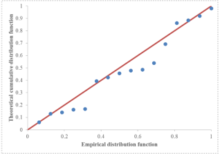
Analysis of the data in Table 3 shows that the calculated p-value is greater than 1 − α = 0.05 (5% significance level). Regarding W_critical, the value is lower than the calculated W. Under these conditions, the experimental values of the acidity constant follow a normal distribution. This normal distribution is confirmed by the scatter plot's alignment along the line y = x (Figure 1).

Download: Download full-size image

Figure 1. P-P plot (pKaexp) of the model.

3.3. Study of the Intercorrelation Between Molecular Descriptors and pKa, and Between Pairs of Molecular Descriptors

First, there should be a linear dependency between the pKa and the calculated molecular descriptors. Furthermore, the correlation between pairs of descriptors must be zero or low to avoid information redundancy. The table below presents the correlation coefficients between the various calculated molecular descriptors and the acidity constant.

Table 4. Descriptor correlation matrix.

Variables	IE	∆_fS⁰	Q	pKa
IE	1.0000
∆_fS⁰	-0.8030	1.0000
Q	0.1852	-0.3650	1.0000
pKa	-0.8691	0.8948	-0.5853	1.0000

The correlation matrix shows that the absolute values of the correlation coefficients (|R|) between pKa and the molecular descriptors are all greater than 0.50. This indicates that the molecular descriptors correlate with the property being modeled. For the pairs (Q, ∆_fS⁰) and (Q, IE), the absolute values of the correlation coefficients are found to be less than 0.50 (|r| < 0.50). These values, all below 0.50, indicate an absence of correlation between these descriptors when considered in pairs. Regarding the molecular descriptors ∆_fS⁰ and IE, it is observed that |r| < 0.90; consequently, these two descriptors are considered to be weakly correlated. In light of the foregoing, these three descriptors can therefore coexist within the same QSPR model. A QSPR model will thus be developed based on these three parameters.

3.4. Development of the QSPR Model: pKa=f (IE, ∆fS0 and Q)

A multiparametric QSPR model based on ionization energy (IE), standard entropy of formation (∆_fS⁰), and the sum of the absolute values of Mulliken charges (Q) was developed using XLSTAT software.

1) Regression equation of the QSPR model

The XLSAT software enabled us to determine the coefficients of the regression equation for the developed QSPR model. The regression coefficients are summarized in Table 5.

Table 5. Model regression coefficient values.

Source	Value	Standard error	t	Pr > \|t\|
Constant	57.3258	4.5374	12.6340	< 0.0001 (***)
IE	-3.7528	0.7087	-5.2952	0.0011 (**)
∆_fS⁰	0.0636	0.0204	3.1153	0.0170 (*)
Q	-0.2167	0.0384	-5.6452	0.0008 (***)

Download: Download full-size image

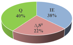
Figure 2. Molecular descriptor contribution diagram.

|t_{critical}| = 2.36

The regression coefficients in Table 5 assigned to the various explanatory variables (molecular descriptors) lead to the following regression equation:

pKa_theo= 57.3258-3.7528IE+0.0636∆_fS⁰-0.2167Q

The regression equation clearly shows that the regression coefficients for ionization energy (IE) and the sum of the absolute values of Mulliken charges (Q) are negative, whereas the coefficient for standard entropy of formation has the opposite sign. Under these conditions, the acidity constant (pKa) decreases as ionization energy and charge decrease; indeed, an increase in these two independent variables (descriptors) leads to a decrease in the acidity constant. Conversely, an increase in standard entropy of formation leads to an increase in the acidity constant. It is also observed that the p-values for the intercept and the charge (Q) fall within the interval

[0; 0.001[

, indicating a highly significant influence (***) on the pKa. As for ionization energy, its p-value falls within the interval

]0, 001; 0.01]

; consequently, its contribution to predicting the property under study is very significant (**). In contrast, the p-value for standard entropy of formation falls within the interval

]0, 01; 0, 05]

, indicating a significant influence on the pKa. Thus, determining these three molecular descriptors is essential for evaluating the acidity constant of the family of molecules studied. The absolute values of the t-statistic and the contribution values reveal that charge Q makes the largest contribution (40.16%), indicating that it is the primary predictive descriptor for the acidity constant of the chlorophenol family studied. Ionization energy contributes 37.67%, while the standard entropy of formation contributes 22.16%. The ranking of the descriptors in descending order of their contribution to the prediction of the acidity constant is as follows:

Q > IE > {∆_{f} S}^{0}

. The contributions of these descriptors can be visualized in the following diagram:

2) Model Analysis of Variance (ANOVA) table

This table allows for the easy calculation of various statistical parameters of the model.

Table 6. Model ANOVA table.

Source	DF	Sum of squares	Mean square	F	Pr > F
Model	3	10.8113	3.6038	93.2600	< 0.0001 (***)
Error	7	0.2705	0.0386
Corrected total	10	11.0818

(***) means "Highly significant"

In Table 6 (ANOVA table), it can be seen that the p-value falls within the range [0, 0.001), indicating that the model's regression equation is highly significant (***) for predicting the acidity constant of the series of molecules studied. This significance is confirmed by the very high value of the Fisher coefficient (F = 93.2600), which far exceeds the significance threshold (F_limit = 4.35). In short, at least one of the explanatory variables is relevant for explaining the dependent variable (acidity constant). A summary of the parameters determined using the ANOVA table is presented in Table 7.

3) Model statistical parameters

Various parameters related to the developed QSPR model were calculated to assess its quality. These parameters are summarized in the table below:

Table 7. Model statistical parameters.

n	R	$R^{2}$	$R_{adjusted}^{2}$	s	F
11	0.9877	0.9756	0.9651	0.1966	93.2600

Table 7 shows a very high correlation coefficient (R = 0.9877), indicating that the acidity constant is strongly correlated with the three selected molecular descriptors. Regarding the adjusted coefficient of determination (

R_{adjusted}^{2}

), it provides greater precision than the standard coefficient of determination (R²). The

R_{adjusted}^{2}

value is 0.9651, revealing that 96.51% of the experimental variance in the acidity constant is explained by the model's descriptors. Furthermore, the low standard deviation (s = 0.1966) indicates a good fit and high prediction reliability. These statistical parameters yielded satisfactory results, demonstrating the high quality of the developed QSPR model. However, validation tests are necessary to avoid overestimating the model's predictive capability regarding truly external molecules.

3.5. Internal Model Validation

Internal validation of a QSPR model applies only to the training set. The validation methods used are Leave-One-Out (LOO) cross-validation and the property randomization test (Y-randomization).

1) Leave-One-Out cross-validation of the model

The LOO cross-validation parameters values are summarized in Table 8.

Table 8. Statistical parameters for the LOO cross-validation of the model.

n	$Q_{LOO}^{2}$	$\overset{̅}{r_{m}^{2} (LOO)}$	${∆ r}_{m}^{2} (LOO)$	PRESS	SDEP
11	0.9395	0.7117	0.0000	0.6699	0.2923

It is noteworthy that the model's LOO cross-validation coefficient is 0.9395, exceeding 0.90. This demonstrates the model's excellence in predicting the acidity constant for the family of molecules under study. Furthermore, the model successfully predicts the acidity constants for approximately 94 of the 100 molecules in the training set. The developed model thus exhibits high predictive capability regarding the molecules in the training set. This result indicates that the developed QSPR model is highly robust showing minimal sensitivity to the Leave-One-Out procedure as evidenced by the very high

Q_{LOO}^{2}

cross-validation coefficient and R² determination coefficient. Regarding the

\overset{̅}{r_{m}^{2} (LOO)}

coefficient, its value is 0.7117 (above 0.50), while the

{∆ r}_{m}^{2} (LOO)

value is below 0.2. Consequently, the developed model is acceptable for predicting the acidity constants of the molecules in the training set. To determine whether the established QSPR model was the result of chance, a randomization test on the property under study was performed.

2) Model Y-randomization test

For the randomization process, a circular permutation (involving 10 iterations) was carried out. A summary of the mean values for the randomization parameters is provided in Table 9.

Table 9. Statistical parameters for the model's internal LOO validation.

Randomized parameter	$R_{r}^{2}$	$s_{r}$	$F_{r}$	${}^{c}{R_{P}^{2}}$
Mean value	0.3718	1.0722	1.0056	0.7675

The mean value of the randomized coefficient of determination (

R_{r}^{2}

) is very low (0.3718), indicating that the regression line equation accounts for only 37.18% of the data point distribution (acidity constant). Furthermore, there is significant dispersion of the data points around the regression line, as confirmed by a high randomized standard deviation (

s_{r}

=1.0722). The very low value of the randomized model's F-statistic (

F_{r} = 1.0056

) indicates that the randomized model equation is not significant. Regarding Todeschini’s corrected parameter (

{}^{c}{R_{P}^{2}}

), its value is 0.7675, which is well above 0.50. Since this parameter exceeds 0.50, it is evident that the developed QSPR model is not the result of chance correlations.

3.6. External Validation of the Model

External validation applies only to the test set. Parameters were determined for this validation, and Tropsha's criteria were verified.

3) Statistical parameters for model external validation

The values of the model's external validation parameters are summarized in Table 10.

Table 10. Statistical parameters for model external validation.

n_ext	$R_{ext}^{2}$	$Q_{ext}^{2}$	$\overset{̅}{r_{m}^{2} (test)}$	${∆ r}_{m}^{2} (test)$	PRESS (test)	RMSEP
5	0.9736	0.6210	0.8194	0.0000	1.9089	0.6179

An analysis of the data in Table 10 indicates that the model possesses acceptable predictive power, evidenced by the high value of the external validation coefficient (

Q_{ext}^{2} = 0.6210

). This implies that, for every 100 molecules in the test set, the model successfully predicts the acidity constants for approximately 62 of them. Furthermore, 97.36% of the experimental variance in the acidity constant is explained by the model's descriptors. Regarding

\overset{̅}{r_{m}^{2} (test)}

, the value exceeds 0.50, while the value for

{∆ r}_{m}^{2} (test)

is below 0.2. Thus, the developed model is acceptable for predicting the property in question for the test set molecules. Additionally, the five Tropsha criteria have been satisfied.

Vérification des critères de Tropsha du modèle

Criterion 1:

R_{ext}^{2} = 0.9736 > 0.70

Criterion 2:

Q_{ext}^{2} = 0.6210 > 0, 60

Criterion 3:

\frac{|R_{ext}^{2} - R_{0}^{2}|}{R_{ext}^{2}} = 0.0258 < 0.1

and

k = 1.0786

with

0.85 < k < 1.15

Criterion 4:

\frac{|R_{ext}^{2} - R_{0}^{' 2}|}{R_{ext}^{2}} = 0.0258 < 0.1

and

k ’ = 0.9259

with

0.85 < k ’ < 1.15

Criterion 5:

|R_{ext}^{2} - R_{0}^{2}| = 0.0251 < 0.3

It is observed that all five of Tropsha’s criteria are met. Consequently, the model performs very well in predicting the acidity constant of the molecules in the test set from the experimental database.

4) Ratio

τ = \frac{{pKa}_{\exp}}{{Pka}_{t h eo}}

of the test set

The model's performance was also evaluated by analyzing the ratio

τ = \frac{{pKa}_{\exp}}{{Pka}_{theo}}

for the test series. The values obtained are summarized in Table 11.

Table 11. Ratio values

τ = \frac{{pKa}_{\exp}}{{pKa}_{t h eo}}

${pKa}_{\exp}$	${pKa}_{theo}$	$τ = \frac{{pKa}_{\exp}}{{pKa}_{theo}}$
9.1000	9.3255	0.9758
6.4000	7.1430	0.8960
6.4000	6.9985	0.9145
7.4000	8.2450	0.8975
5.3000	5.7833	0.9164

Analysis of Table 11 shows that the values of the ratio

τ = \frac{{pKa}_{\exp}}{{pKa}_{theo}}

are essentially equal to unity. This demonstrates that the model performs very well in predicting the acidity constant for the series of molecules studied and can be used to predict values for other molecules in the same family.

5) Comparison between model-predicted values and experimental values of the acidity constant for the test set

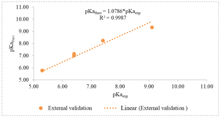
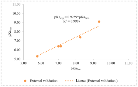
The theoretical pKa values were compared with the experimental values based on the regression constants from the pKa_theo=f(pKa_exp) plots in Figure 3 and the pKa_exp=f(pKa_theo) plots in Figure 4.

Download: Download full-size image

Figure 3. Plot of pKatheo=f(pKaexp) for the model test series (intercept = 0).

Download: Download full-size image

Figure 4. Plot of pKaexp=f(pKatheo) for the model test series (intercept = 0).

Based on Figures 3 and 4, the slope values k = 1.0786 and k’ = 0.9259 are very close to unity. This indicates that the calculated pKa value is very close to the experimental value (pKa_theo=f(pKa_exp)), resulting in a ratio close to unity. The external validation results further demonstrate that the model performs very well in predicting the pKa of the studied series of molecules. It can be effectively used to predict the pKa of new chlorophenols falling within its applicability domain.

3.7. Correlation Between Model-predicted Values and Experimental Values of the Acidity Constant

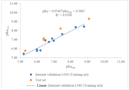
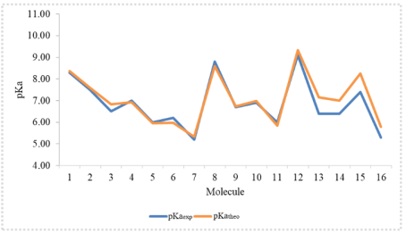
The distribution of data points around the regression line in Figure 5 reveals a strong linear correlation between the model-predicted pKa values and the experimental values. Figure 6 shows a similarity between the curves representing the model-predicted values and the experimental values, particularly for the test set. Consequently, these graphs confirm that the model is validated and acceptable for pKa prediction. This also reflects the suitability of the level of theory employed to develop this QSPR model.

Download: Download full-size image

Figure 5. PKatheo-pKaexp scatter plot of the model.

Download: Download full-size image

Figure 6. Similarity curve between model-predicted pKa values and experimental pKa values.

3.8. Normality Test for Model Data

The Shapiro-Wilk test was used to verify the normality of the data derived from the model. The test parameters are summarized in Table 12.

Table 12. Shapiro-Wilk test parameters for the model.

W	W_critique	p-value	$1 - α$
0.9496	0.8870	0.4837	0.05

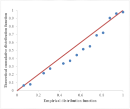
Analyse of the values in Table 12 shows that the calculated p-value is greater than 1 − α = 0.05 (5% significance level). Regarding W-critical, the value is lower than the calculated W. Consequently, the normality hypothesis is consistent with our data. This normal distribution is confirmed by the scatter plot's alignment along the first bisector (the line defined by y = x) (Figure 7).

Download: Download full-size image

Figure 7. P-P plot (pKatheo) of the model.

4. Conclusion

This study investigated the predicted variation of the acidity constant of sixteen (16) chlorophenols based on quantum chemical descriptors. A multiparametric QSPR model was developed, incorporating ionization energy (IE), standard entropy of formation (∆_fS⁰), and the sum of the absolute values of Mulliken charges (Q). The model demonstrates highly satisfactory statistical and validation parameters,

R^{2}

=0.9756;

R_{adjusted}^{2}

=0.9651; s=0.1966; F=93.2600; Q²_LOO=0.9395;

\overset{̅}{r_{m}^{2} (LOO)}

=0.7117;

{∆ r}_{m}^{2} (LOO)

= 0.0000);

R_{ext}^{2}

=0.9736; Q²_ext=0.6210;

\overset{̅}{r_{m}^{2} (test)}

=0.8194;

{∆ r}_{m}^{2} (test)

= 0.0000. These various parameters demonstrate that the developed QSPR model is validated and performs well in predicting the acidity constant, making it an acceptable predictive model. Consequently, it can now be used to predict the acidity constant of future chlorophenols from the same family that fall within its applicability domain. Therefore, future work will involve using this model to design new chlorophenols with desired acidity constants.

Abbreviations

QSPR	Quantitative Structure-Property Relationship
QSAR	Quantitative Structure-Activity Relationship
MLR	Multiple Linear Regression
TSS	Total Sum of Squares
ESS	Extended Sum of Squares
RSS	Residual Sum of Squares
PRESS	Prediction Sum of Squares
SDEP	Standard Deviation of Error of Prediction
HOMO	Highest Occupied Molecular Orbital
IE	Ionization Energy

Author Contributions

Fatogoma Diarrassouba: Conceptualization

Affoue Lucie Bede: Data curation, Methodology

Kafoumba Bamba: Formal Analysis

Nahosse Ziao: Writing – review & editing

Conflicts of Interest

The authors declare no conflicts of interest.

References

[1]	Teodora Ivanciuc, Ovidiu Ivanciuc and Douglas J. Klein, Prediction of Environmental Properties for Chlorophenols with Posetic Quantitative Super-Structure/Property Relationships (QSSPR), International Journal of Molecular Sciences, 2006, 358-374, https://doi.org/10.3390/i7090358
[2]	Kaise, K. L. E., Organic Contaminants in the Environment: Research Progress and Needs, Environment International, 1984, 241-250, https://doi.org/10.1016/0160-4120(84)90241-1
[3]	Keith, Larry H.; Telliard, William A., Priority Pollutants: I. A Perspective View, Environmental Science and Technology, 1979, 416-423, https://doi.org/10.1021/es60152a601
[4]	Marianna Czaplicka. (2004). Sources and transformations of chlorophenols in the natural environment, Science of the Total Environment, 2004, 21-39, https://doi.org/10.1016/j.scitotenv.2003.09.015
[5]	European Parliament and Council of the European Union (2006) Regulation (EC) No 1907/2006 of the European Parliament and of the Council of 18 December 2006 concerning the registration, evaluation, authorisation and restriction of chemicals (REACH), establishing a European Chemicals Agency, amending Directive 1999/ 45/EC and repealing Council Regulation (EEC) No 793/93 and Commission Regulation (EC) No 1488/94 as well as Council Directive 76/769/EEC and Commission Directives 91/155/EEC, 93/67/EEC, 93/105/EC and 2000/21/EC. Official Journal of the European Union, 2006, L 396, 1-849. https://eurlex.europa.eu/legal-content/EN/TXT/?uri=CELEX:32006R1907
[6]	Margossian, N. (2008) Le règlement REACH—La règlementation européenne sur les produits chimiques. Dunod.
[7]	Sangster, J. Octanol-water Partition Coefficients of Simple Organic Compounds. Journal of Physical and Chemical Reference Data, 1989, 1111-1229. https://doi.org/10.1063/1.555833
[8]	Roy, K., Kar, S. and Das, R. N., Understanding the Basics of QSAR for Applications in Pharmaceutical Sciences and Risk Assessment, Academic Press, 2015.
[9]	Pierre-André Cornillon, Eric Matzner-Løber, Régression avec R, Springer-Verlag France, 2011.
[10]	Gramatica, P., Giani, E. and Papa, E., Statistical External Validation and Consensus Modeling: A QSPR Case Study for Koc Prediction. Journal of Molecular Graphics and Modelling, 2007, 755-766. https://doi.org/10.1016/j.jmgm.2006.06.005
[11]	Kahn, I., Fara, D., Karelson, M., Maran, U. and Andersson, P. L., QSPR Treatment of the Soil Sorption Coefficients of Organic Pollutants. Journal of Chemical Information and Modeling, 2004, 94-105. https://doi.org/10.1021/ci0498766
[12]	R Dennington, T Keith and J Millam., GaussView Version 5, Semichem Inc., Shawnee Mission, KS, 2009.
[13]	Frisch, M. J., Trucks, G. W., Schlegel, H. B., Scuseria, G. E., Robb, M. A., Cheeseman, J. R., et al. Gaussian 09, Revision A. 02. Gaussian, Inc., 2009.
[14]	ACDLABS 10, Advanced Chemistry Development Inc., Toronto, ON, Canada, 2015.
[15]	Snedecor G. W., Cochran W. G., Statistical methods, Wiley-Blackwell, 1991, 503 p.
[16]	Vessereau A. Méthodes statistiques en biologie et en agronomie. Lavoisier (Tec & Doc), Paris, 1988, 538p.
[17]	Trinajstič, N., Nikolič, S., Basak, S. C. and Lukovits, I. (2001) Distance Indices and Their Hyper-Counterparts: Intercorrelation and Use in the Structure-Property Modeling. SAR and QSAR in Environmental Research, 2001, 31-54. https://doi.org/10.1080/10629360108035370
[18]	Koopmans, T., Über die Zuordnung von Wellenfunktionen und Eigenwerten zu den Einzelnen Elektronen Eines Atoms. Physica, 1934, 104-113. https://doi.org/10.1016/s0031-8914(34)90011-2
[19]	M. W. Chase, Jr., C. A. Davies, J. R. Downey, Jr., D. J. Frurip, R. A. McDonald, and A. N. Syverud, J. Phys. Ref. Data 14 Suppl. No. 1; (JANAF Thermochemical Tables), 1985.
[20]	Ochterski, J. W. (2000). Thermochemistry in Gaussian [Technical note]. Gaussian, Inc., 2000.
[21]	Chatterje S. and Hadi A. S., Regression Analysis by Example. 4th Edition, John Wiley & Sonc, Inc., Hoboken, 2006, 366 p,
[22]	A. F. Siegel, Practical Business Statistics, IRWIN, 3rd edition, 1997.
[23]	P. Besse., Pratique de la modélisation statistique, Publications du laboratoire de statistique et Probabilité, 2003.
[24]	Cook, R. D. and Weisberg, S. (1994). An Introduction to Regression Graphics. Wiley, 1994, 265 p. https://doi.org/10.1002/9780470316863
[25]	Golbraikh, A. and Tropsha, A. (2002) Beware of Q2! Journal of Molecular Graphics and Modelling, 2002, 269-276, https://doi.org/10.1016/s1093-3263(01)00123-1
[26]	L. Erikson, J. Jaworska, A. Worth, M. Cromin, R. M. Mc Dowell, P. Gramatica., Methods for reliability, uncertainty assessment, and applicability evaluations of regression based and classification QSPRs, Environmental Health Perspective, 2003, 1361-1375 https://doi.org/10.1289/ehp.5758
[27]	Mitra, I., Saha, A. and Roy, K. (2010) Exploring Quantitative Structure-Activity Relationship Studies of Antioxidant Phenolic Compounds Obtained from Traditional Chinese Medicinal Plants. Molecular Simulation, 2010, 1067-1079. https://doi.org/10.1080/08927022.2010.503326
[28]	Pratim Roy, P., Paul, S., Mitra, I. and Roy, K., On Two Novel Parameters for Validation of Predictive QSAR Models. Molecules, 2009, 1660-1701. https://doi.org/10.3390/molecules14051660
[29]	Consonni, V., Ballabio, D. and Todeschini, R. (2010) Evaluation of Model Predictive Ability by External Validation Techniques. Journal of Chemometrics, 2010, 194-201. https://doi.org/10.1002/cem.1290
[30]	Roy, K., Mitra, I., Kar, S., Ojha, P. K., Das, R. N. and Kabir, H., Comparative Studies on Some Metrics for External Validation of QSPR Models. Journal of Chemical Information and Modeling, 2012, 396-408. https://doi.org/10.1021/ci200520g
[31]	Tropsha, A., Gramatica, P. and Gombar, V. K. (2003) The Importance of Being Earnest: Validation Is the Absolute Essential for Successful Application and Interpretation of QSPR Models. QSAR & Combinatorial Science, 2003, 69-77. https://doi.org/10.1002/qsar.200390007
[32]	Shapiro, S. S. and Wilk, M. B. An Analysis of Variance Test for Normality (Complete Samples). Biometrika, 1965, 591-611. https://doi.org/10.1093/biomet/52.3-4.591

Cite This Article

Plain Text BibTeX RIS

APA Style

Diarrassouba, F., Bede, A. L., Bamba, K., Ziao, N. (2026). Study of the Predicted Variation of the Acidity Constant (pKa) of a Family of Chlorophenols as a Function of Quantum Chemical Descriptors. International Journal of Environmental Chemistry, 10(2), 19-33. https://doi.org/10.11648/j.ijec.20261002.11

Copy | Download

ACS Style

Diarrassouba, F.; Bede, A. L.; Bamba, K.; Ziao, N. Study of the Predicted Variation of the Acidity Constant (pKa) of a Family of Chlorophenols as a Function of Quantum Chemical Descriptors. Int. J. Environ. Chem. 2026, 10(2), 19-33. doi: 10.11648/j.ijec.20261002.11

Copy | Download

AMA Style

Diarrassouba F, Bede AL, Bamba K, Ziao N. Study of the Predicted Variation of the Acidity Constant (pKa) of a Family of Chlorophenols as a Function of Quantum Chemical Descriptors. Int J Environ Chem. 2026;10(2):19-33. doi: 10.11648/j.ijec.20261002.11

Copy | Download

@article{10.11648/j.ijec.20261002.11,
  author = {Fatogoma Diarrassouba and Affoue Lucie Bede and Kafoumba Bamba and Nahosse Ziao},
  title = {Study of the Predicted Variation of the Acidity Constant (pKa) of a Family of Chlorophenols as a Function of Quantum Chemical Descriptors},
  journal = {International Journal of Environmental Chemistry},
  volume = {10},
  number = {2},
  pages = {19-33},
  doi = {10.11648/j.ijec.20261002.11},
  url = {https://doi.org/10.11648/j.ijec.20261002.11},
  eprint = {https://article.sciencepublishinggroup.com/pdf/10.11648.j.ijec.20261002.11},
  abstract = {The acidity constant, or acid dissociation constant (Ka), is a quantitative measure of the strength of an acid in solution. It reflects the tendency of an acid to dissociate and release a proton (H⁺ or H3O+) to water. It serves as the equilibrium constant for the dissociation reaction of an acidic species within the context of acid-base reactions. The higher the value of Ka, the greater the extent of molecular dissociation in solution, and consequently, the stronger the acid. Since Ka values can span several orders of magnitude, a logarithmic scale known as pKa is frequently used. In this study, we conducted a predictive analysis of the acidity constant of sixteen (16) chlorophenols based on quantum-chemical molecular descriptors. The results obtained are satisfactory and promising regarding the prediction and explanation of the acidity constant for this family of molecules. A QSPR (Quantitative Structure-Property Relationship) model linking the acidity constant (pKa) to three molecular descriptors was developed. These molecular descriptors namely ionization energy (IE), standard entropy of formation (∆fS0), and the sum of the absolute values of Mulliken charges (Q) enable the explanation and prediction of the acidity constant for this family of molecules. This model exhibited highly satisfactory statistical and validation parameters. They indicate that the developed QSPR model is validated and performs well in predicting the acidity constant. It can therefore be used to effectively predict the acidity constant of other molecules within its applicability domain at a 95% confidence level.},
 year = {2026}
}

Copy | Download

TY - JOUR
T1 - Study of the Predicted Variation of the Acidity Constant (pKa) of a Family of Chlorophenols as a Function of Quantum Chemical Descriptors
AU - Fatogoma Diarrassouba
AU - Affoue Lucie Bede
AU - Kafoumba Bamba
AU - Nahosse Ziao
Y1 - 2026/10/28
PY - 2026
N1 - https://doi.org/10.11648/j.ijec.20261002.11
DO - 10.11648/j.ijec.20261002.11
T2 - International Journal of Environmental Chemistry
JF - International Journal of Environmental Chemistry
JO - International Journal of Environmental Chemistry
SP - 19
EP - 33
PB - Science Publishing Group
SN - 2640-1460
UR - https://doi.org/10.11648/j.ijec.20261002.11
AB - The acidity constant, or acid dissociation constant (Ka), is a quantitative measure of the strength of an acid in solution. It reflects the tendency of an acid to dissociate and release a proton (H⁺ or H3O+) to water. It serves as the equilibrium constant for the dissociation reaction of an acidic species within the context of acid-base reactions. The higher the value of Ka, the greater the extent of molecular dissociation in solution, and consequently, the stronger the acid. Since Ka values can span several orders of magnitude, a logarithmic scale known as pKa is frequently used. In this study, we conducted a predictive analysis of the acidity constant of sixteen (16) chlorophenols based on quantum-chemical molecular descriptors. The results obtained are satisfactory and promising regarding the prediction and explanation of the acidity constant for this family of molecules. A QSPR (Quantitative Structure-Property Relationship) model linking the acidity constant (pKa) to three molecular descriptors was developed. These molecular descriptors namely ionization energy (IE), standard entropy of formation (∆fS0), and the sum of the absolute values of Mulliken charges (Q) enable the explanation and prediction of the acidity constant for this family of molecules. This model exhibited highly satisfactory statistical and validation parameters. They indicate that the developed QSPR model is validated and performs well in predicting the acidity constant. It can therefore be used to effectively predict the acidity constant of other molecules within its applicability domain at a 95% confidence level.
VL - 10
IS - 2
ER -

Copy | Download

Author Information

Fatogoma Diarrassouba

Faculty of Fundamental and Applied Sciences, Nangui Abrogoua University, Abidjan, Côte d’Ivoire;Faculty of Science and Technology, Alassane Ouattara University, Bouake, Côte d’Ivoire

Contact Email
Affoue Lucie Bede

Faculty of Sciences of the Structures of Matter and Technology, Félix Houphouët-Boigny University, Abidjan, Côte d’Ivoire
Kafoumba Bamba

Faculty of Fundamental and Applied Sciences, Nangui Abrogoua University, Abidjan, Côte d’Ivoire
Nahosse Ziao

Faculty of Fundamental and Applied Sciences, Nangui Abrogoua University, Abidjan, Côte d’Ivoire;Ivorian Research Group on Disease Modeling, Nangui Abrogoua University, Abidjan, Côte d’Ivoire

Download PDF

Submit an Article

Plain Text BibTeX RIS

APA Style

Diarrassouba, F., Bede, A. L., Bamba, K., Ziao, N. (2026). Study of the Predicted Variation of the Acidity Constant (pKa) of a Family of Chlorophenols as a Function of Quantum Chemical Descriptors. International Journal of Environmental Chemistry, 10(2), 19-33. https://doi.org/10.11648/j.ijec.20261002.11

Copy | Download

ACS Style

Diarrassouba, F.; Bede, A. L.; Bamba, K.; Ziao, N. Study of the Predicted Variation of the Acidity Constant (pKa) of a Family of Chlorophenols as a Function of Quantum Chemical Descriptors. Int. J. Environ. Chem. 2026, 10(2), 19-33. doi: 10.11648/j.ijec.20261002.11

Copy | Download

AMA Style

Diarrassouba F, Bede AL, Bamba K, Ziao N. Study of the Predicted Variation of the Acidity Constant (pKa) of a Family of Chlorophenols as a Function of Quantum Chemical Descriptors. Int J Environ Chem. 2026;10(2):19-33. doi: 10.11648/j.ijec.20261002.11

Copy | Download

@article{10.11648/j.ijec.20261002.11,
  author = {Fatogoma Diarrassouba and Affoue Lucie Bede and Kafoumba Bamba and Nahosse Ziao},
  title = {Study of the Predicted Variation of the Acidity Constant (pKa) of a Family of Chlorophenols as a Function of Quantum Chemical Descriptors},
  journal = {International Journal of Environmental Chemistry},
  volume = {10},
  number = {2},
  pages = {19-33},
  doi = {10.11648/j.ijec.20261002.11},
  url = {https://doi.org/10.11648/j.ijec.20261002.11},
  eprint = {https://article.sciencepublishinggroup.com/pdf/10.11648.j.ijec.20261002.11},
  abstract = {The acidity constant, or acid dissociation constant (Ka), is a quantitative measure of the strength of an acid in solution. It reflects the tendency of an acid to dissociate and release a proton (H⁺ or H3O+) to water. It serves as the equilibrium constant for the dissociation reaction of an acidic species within the context of acid-base reactions. The higher the value of Ka, the greater the extent of molecular dissociation in solution, and consequently, the stronger the acid. Since Ka values can span several orders of magnitude, a logarithmic scale known as pKa is frequently used. In this study, we conducted a predictive analysis of the acidity constant of sixteen (16) chlorophenols based on quantum-chemical molecular descriptors. The results obtained are satisfactory and promising regarding the prediction and explanation of the acidity constant for this family of molecules. A QSPR (Quantitative Structure-Property Relationship) model linking the acidity constant (pKa) to three molecular descriptors was developed. These molecular descriptors namely ionization energy (IE), standard entropy of formation (∆fS0), and the sum of the absolute values of Mulliken charges (Q) enable the explanation and prediction of the acidity constant for this family of molecules. This model exhibited highly satisfactory statistical and validation parameters. They indicate that the developed QSPR model is validated and performs well in predicting the acidity constant. It can therefore be used to effectively predict the acidity constant of other molecules within its applicability domain at a 95% confidence level.},
 year = {2026}
}

Copy | Download