ALE Numerical Simulation for a Rigid Body Rotation About a Fixed Axis in a Incompressible Viscous Fluid

Wan Il Kim; Jae Wan Jo; Wan Hui Jo; Myong Chol Ri; Song Bom Pyon

doi:doi:10.11648/j.ijfmts.20251104.11

Research Article |

| Peer-Reviewed

ALE Numerical Simulation for a Rigid Body Rotation About a Fixed Axis in a Incompressible Viscous Fluid

Wan Il Kim, Jae Wan Jo, Wan Hui Jo, Myong Chol Ri^*

, Song Bom Pyon

Published in International Journal of Fluid Mechanics & Thermal Sciences (Volume 11, Issue 4)

Received: 28 June 2025 Accepted: 29 July 2025 Published: 10 October 2025

Views: Downloads:

Download PDF

Share This Article

Twitter
Linked In
Facebook

Abstract

An efficient numerical method is presented in this paper. It combines a unique ALE formulation with an adaptive time algorithm based on a Courant-Friedrichs-Levy (CFL) type condition to simulate fluid and rigid body interactions. The ALE differential formulation includes the geometric conservation law (GCL) which has the mesh velocity as a variable. In the adaptive time algorithm, the time step selection is based on the CFL type condition which is estimated by the difference between the fluid and mesh velocity. With the adaptive algorithm, the numerical simulations of incompressible viscous flow around moving bodies when the motion of the bodies is not known in advance are stable. To validate the proposed method, only the body rotation about a fixed axis in a incompressible viscous fluid is considered because it causes the large deformation of mesh. The harmonic and damped vibrations of a physical pendulum in the air are tested and the opening of a swing check valve plate is simulated to determine its local resistance characteristics in comparison with experimental data. The numerical simulations show that when a rigid body rotates in an incompressible fluid, the distortion of the mesh element is not significant and the numerical results agree with the experimental data.

Published in	International Journal of Fluid Mechanics & Thermal Sciences (Volume 11, Issue 4)
DOI	10.11648/j.ijfmts.20251104.11
Page(s)	62-75
Creative Commons	This is an Open Access article, distributed under the terms of the Creative Commons Attribution 4.0 International License (http://creativecommons.org/licenses/by/4.0/), which permits unrestricted use, distribution and reproduction in any medium or format, provided the original work is properly cited.
Copyright	Copyright © The Author(s), 2025. Published by Science Publishing Group

Keywords

Adaptivity, Arbitrary Lagrangian-Eulerian, Courant-Friedrichs-Levy (CFL), Rigid Body Rotation

1. Introduction

Fluid and body interactions in which the motion of the body is not known in advance but results from the hydrodynamical application and external forces such as gravity can be found in many engineering applications

[1-4, 17-19]

. Due to the complication of these problems, measurements are sometimes limited for capturing necessary information of flow phenomena such as the local resistance characteristic at the opening interval of the swing check valve which is used in underwater exhaustion or fire extinguishing systems. In this case, the numerical simulation gives us another choice to understand flow phenomena and engineering improvement such as reducing cost, improving performance or reducing failures.

The numerical simulation of fluid and rigid body system rely on the Eulerian method and the arbitrary Lagrangian-Eulerian (ALE) method. The Eulerian method includes immersed boundary method

[5]

, immersed interface method

[6]

, fictitious domain method

[7]

and so on. The Eulerian method has the main advantage of solving problems with variable domains on a fixed regular grid without body-conformal meshing, but its drawbacks are the challenging interface resolution and imposition of boundary condition on the interface. The applications of fluid and rigid body system by the Eulerian method are commonly limited to the flow solutions over a cylinder or a sphere at the low Reynolds numbers. In the ALE method, where the grids can be moved in any arbitrarily specified way independent of the flow motions, it is easy to analyze interfaces and to impose directly boundary conditions on the interface, and hence one can obtain higher accurate results for the interface dynamics in comparison with the Eulerian approach. Therefore, the ALE method is applied in many practical problems

[8]

In ALE related works

[8, 16]

, the ALE differential formations of the hydrodynamic governing equations are differently given, which is confusing. But their integral forms are similar. Also, apart from the ALE differential formulation, the bulk of the work focused on the discrete geometric conservation law (DGCL) which states that the computation of the geometric parameters must be performed in such a way that, independently of the mesh motion, the resulting numerical scheme preserves the state of a uniform flow.

This paper presents a unique ALE differential formulation for the incompressible viscous flows with variable domains. This formulation includes the differential form of the geometric conservation law (GCL) which has the mesh velocity as a variable. The DGCL results from the differential GCL.

The key of the ALE numerical simulation is to specify the mesh velocity in such a way that the quality of moving mesh, that is, the DGCL is satisfied. If the mesh has the bad quality such as the degeneration of mesh cells or the mesh distortion due to crossing or stretching of mesh edges, the accuracy of solution drops and the solution is unstable and thus, the solution process fails. The stability of ALE schemes has been studied in several works

[8]

. In

[11]

, the authors proposed an adaptive algorithm for time integration of fluid-structure integration problems, in which the time step selection is based on a local error estimate, an error controller and a step rejection mechanism. The mesh velocity is affected by the body velocity which is coupled with the fluid velocity through the hydrodynamical force, and hence the reasonable mesh velocity is naturally related to the fluid velocity. On a fixed mesh, the stability of Eulerian explicit schemes requires the restriction of time step by the traditional CFL condition, which does not include the mesh velocity. Nevertheless, in

[12, 13, 19]

, the authors used such CFL type conditions without the mesh velocity for ALE numerical simulations. In

[9]

, the authors performed the nonlinear stability analysis of the ALE schemes based on the CFL type conditions which is estimated by the difference between the fluid and mesh velocities. But they construct the special moving meshes by which it is difficult to solve the ALE problems in which the motion of the body is not known in advance.

This paper presents an adaptive time algorithm for the numerical simulation of the incompressible viscous flow past moving rigid bodies when the motion of the bodies is not known in advance but results from the hydrodynamical coupling and external forces such as gravity, in which the time step selection is based on a CFL type condition similar to the Eq. (36) in

[8]

. In numerical simulations, where the differential GCL with the mesh velocity as a variable is included in the formulation of ALE problem and the mesh and fluid velocity are coupled through the CFL type condition, the stability of the transient ALE solution will be naturally justified.

In this paper, to validate the proposed method, the pure body rotation about a fixed axis in a incompressible viscous fluid is considered because it causes the large deformation of mesh. The harmonic and damped vibrations of physical pendulum in the air are tested and the opening of a swing check valve is simulated to determine its local resistance characteristics in compression with the experimental data

[14, 18, 20]

The paper is organized as follows. In Section 2 we present the ALE differential formulation for the incompressible viscous flows with variable domains and the fully coupled equations for the fluid and body interaction problems in which the body only rotates about a fixed axis. In Section 3 the discretization by the cell-centered finite volume method for the coupled equations is addressed, and in Section 4 the spring analogy

[15]

with no damping is used to move the grid points and the adaptive algorithm for time integration of fluid and body interaction problems is given based on a CFL type condition. In Section 5, numerical examples of the body rotation about a fixed axis in a fluid domain are given. Finally, the concluding remarks are presented in Section 6.

2. Fully Coupled Equations for Fluid and Body Interaction Problems

Here, we present the ALE differential formulation for the incompressible viscous flows with variable domains and the fully coupled equations for the fluid and body interaction problems in which the body only rotates about a fixed axis.

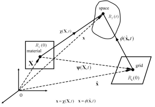
2.1. ALE Kinematic Description

In the ALE description of motion, as shown in Figure 1, neither the material

{\hat{R}}_{X}

nor the spatial

R_{x}

configuration is taken as the referential system

R_{\hat{x}}

, where reference coordinate

\hat{x}

is introduced to identify the mesh points.

A particle motion may be considered to be resulted with

X

via

χ (X, t)

, or via in a combined motion of

ψ (X, t)

and

ϕ (\hat{x}, t)

. Different views of motion can be made, depending upon which coordinates or descriptions are used

[3]

In the Lagrangian description, the velocity of the particle observed by an observer standing at O is

u = {\frac{\partial x}{\partial t}|}_{X} = {\frac{\partial χ (X, t)}{\partial t}|}_{X} = u (X, t) .

(1)

In the Eulerian description, the observer, standing still at O, with his eyes focused at position

x

, will observe a velocity at

x

and at

t

u (x, t)

u = {\frac{\partial x}{\partial t}|}_{X} = {\frac{\partial χ (X, t)}{\partial t}|}_{X} = {\frac{\partial χ (χ^{- 1} (x, t), t)}{\partial t}|}_{X} = u (x, t) .

(2)

Download: Download full-size image

Figure 1. Various configurations used for the ALE description.

In the ALE description, if the observer stands at

\hat{x}

, with his eyes focused at

x

, he will observe a velocity at

x

and at

t

v (\hat{x}, t)

v = {\frac{\partial ϕ (\hat{x}, t)}{\partial t}|}_{\hat{x}} = v (\hat{x}, t)

(3)

Again, the observer, standing at O, with his eyes focused at position

x

, will observe a velocity at

x

and at

t

v (x, t)

v = {\frac{\partial x}{\partial t}|}_{\hat{x}} = {\frac{\partial ϕ (\hat{x}, t)}{\partial t}|}_{\hat{x}} = {\frac{\partial ϕ (ϕ^{- 1} (x, t), t)}{\partial t}|}_{\hat{x}} = v (x, t)

(4)

In order to express the conservation law in an ALE reference system, the material time derivatives inherent to conservation law, must be related to referential time derivatives. The relationships between the time derivatives of physical quantity

f

are

\frac{df}{dt} {= \frac{\partial f}{\partial t}|}_{X} = {\frac{\partial f}{\partial t}|}_{x} + u \cdot \nabla_{x} f

(5)

{\frac{\partial f}{\partial t}|}_{\hat{x}} = {\frac{\partial f}{\partial t}|}_{x} + v \cdot \nabla_{x} f

(6)

{\frac{\partial f}{\partial t}|}_{X} = {\frac{\partial f}{\partial t}|}_{\hat{x}} + (u - v) \cdot \nabla_{x} f

(mixed ALEform)(7)

{\frac{\partial f}{\partial t}|}_{X} = {\frac{\partial f}{\partial t}|}_{\hat{x}} + J^{- 1} (u - v) \cdot \nabla_{\hat{x}} f

.(pure ALEform)(8)

where

J = \partial x / \partial \hat{x}, J = \det (J)

and

\nabla_{\hat{x}} = J \nabla_{x}

.(9)

2.2. Differential ALE Form of the Incompressible Flow Equations

Denoting a variable fluid domain by

Ω (t)

with the boundary being

\partial Ω (t)

and a rigid body domain by

B (t)

with the boundary

\partial B (t)

at a given instant

t \in [0, T]

, the unsteady incompressible Navier-Stokes equations in

Ω (t)

are given in the Eulerian form by

\frac{\partial ρ}{\partial t} + \nabla \cdot (ρ u) = 0

(10)

\frac{\partial (ρ u)}{\partial t} + \nabla \cdot (ρ uu) = - \nabla p + \nabla \cdot τ

(11)

Where,

u

is the velocity vector,

ρ

is the density,

p

is the pressure. For Newtonian fluids, the viscous stress tensor is given by

τ = μ (\nabla u + (\nabla u)^{T})

where

μ

is the dynamic viscosity.

Now, we will transform Eqs. (10) and (11) into ALE form. The time derivative of the

J

in Eq. (9) in the referential frame

R_{\hat{x}}

(or

Ω (\hat{x}, 0)

) with

\hat{x}

fixed is given by

\dot{J} = {\frac{\partial J}{\partial t}|}_{\hat{x}} = Jtr (J^{- 1} \dot{J}) = Jtr (J^{- 1} \nabla vJ) = J (J^{- 1} : \nabla vJ) = J (\nabla vJ : J^{- 1}) = Jtr (\nabla v) = J \nabla \cdot v

(12)

where

\nabla = \nabla_{x} = \partial / \partial x

and (:) is the double contraction. Using Eqs. (7) and (12), Eq. (10) can be written in the mixed ALE form. Note that the mixed form is convenient to obtain equations in integral form

\frac{\partial ρ}{\partial t} + \nabla \cdot (ρu) = {\frac{\partial ρ}{\partial t}|}_{x} + \nabla_{x} \cdot (ρu) = \frac{dρ}{dt} + ρ \nabla_{x} \cdot u

= {\frac{\partial ρ}{\partial t}|}_{X} + ρ \nabla_{x} \cdot u = {\frac{\partial ρ}{\partial t}|}_{\hat{x}} + (u - v) \cdot \nabla_{x} ρ + ρ \nabla_{x} \cdot u = \frac{1}{J} [{J \frac{\partial ρ}{\partial t}|}_{\hat{x}} + J (u - v) \cdot \nabla_{x} ρ + Jρ \nabla_{x} \cdot u + ρ {\frac{\partial J}{\partial t}|}_{\hat{x}} - ρ {\frac{\partial J}{\partial t}|}_{\hat{x}}]

= \frac{1}{J} [({J \frac{\partial ρ}{\partial t}|}_{\hat{x}} + ρ {\frac{\partial J}{\partial t}|}_{\hat{x}}) + J (u - v) \cdot \nabla_{x} ρ + Jρ \nabla_{x} \cdot u - ρJ \nabla_{x} \cdot v]

= \frac{1}{J} [{\frac{\partial (ρJ)}{\partial t}|}_{\hat{x}} + J \nabla_{x} \cdot [ρ (u - v)]] = \frac{1}{J} [{\frac{\partial (ρJ)}{\partial t}|}_{\hat{x}} + J \nabla \cdot [ρ (u - v)]] = 0

(13)

From Eq. (12), Eq. (13) for the incompressible fluid results in

\nabla \cdot u = 0

(14)

Similar to Eq. (13), Eq. (11) can be written in the ALE form by

{\frac{\partial (Jρu)}{\partial t}|}_{\hat{x}} + J \nabla \cdot [ρ (u - v) u] = - J \nabla p + J \nabla \cdot τ

.(15)

Summarizing Eqs. (12)-(15), we have the ALE differential formulation for the incompressible viscous flows in variable domains.

{\frac{\partial J}{\partial t}|}_{\hat{x}} - J \nabla \cdot v = 0

(GCL in differentialform)(16)

J \nabla \cdot u = 0

(17)

{\frac{\partial (Jρu)}{\partial t}|}_{\hat{x}} + J \nabla \cdot [ρ (u - v) u] = - J \nabla p + J \nabla \cdot τ

(18)

We will call Eq. (16) the GCL in differential form. Because the mesh velocity

v

is the unknown quantity, Eq. (16) should be included in the ALE formulation. In Section 4, we will describe the method that combines the mesh velocity with the flow velocity through a CFL type condition for any incompressible flows.

Note that the continuity equation, Eq. (14) was replaced with Eq. (17) for its integral form.

2.3. Rigid Body Rotation About a Fixed Axis

In the work, the pure body rotation about a fixed axis in a incompressible viscous fluid is considered because it causes the large deformation of mesh. To do this, the following motion equation of the rigid body is coupled with Eqs. (16)-(18).

I \frac{dω}{dt} = M + M_{f}

(19)

where

ω

is the angular velocity vector of the body,

I

the axial moment of inertia of the body,

M

the moment duo to external forces such as the gravity, and

M_{f}

the hydrodynamic moment acting on the body. The hydrodynamic moment is given by.

M_{f} = - \int_{\partial B} r_{\partial B} \times (τ - pI) nd (\partial B)

(20)

where

n

is the unit normal vector on the surface of the body pointing into the body and

r_{\partial B}

is the position vector from the fixed axis to the body surface.

The boundary of the fluid domain

Ω (t)

can be decomposed into three nonoverlapping sections:

(\partial Ω)_{u}

(\partial Ω)_{p}

, and

\partial B

. On these boundary sections the following boundary conditions are imposed.

u = u_{b}

,on

(\partial Ω)_{u}

(21)

p = p_{b}

,on

(\partial Ω)_{p}

(22)

u (x) = ω \times r_{\partial B} (x)

,for

\forall x \in \partial B (t)

(23)

Where,

u_{b}

and

p_{b}

are the prescribed velocity and pressure, respectively.

The initial conditions for the flow field and the body variables are

u (0) = u_{0}

and

p = p_{0}

,in

Ω (0)

(24)

θ (0) = θ_{0}, ω (0) = ω_{0}

(25)

3. Finite Volume Discretization

3.1. Integral Form of Eqs. (16)-(18)

We assume that the initial fluid domain

Ω (\hat{x}, 0)

is discretized with control volumes or cells. Integrating Eqs. (16)-(18) over any control volume

V (0)

in the initial mesh, then getting integrals over the control volume

V (t)

in a given instant

t

by considering the relation

dV = d V_{x} = Jd V_{\hat{x}}

from Eq. (9), and finally, integrating them by parts, we get

\frac{d}{dt} \int_{V (t)} dV = \int_{\partial V (t)} v \cdot n dA

(26)

\int_{\partial V (t)} u \cdot n ​​ dA ​​​​​ = 0

(27)

\frac{d}{dt} \int_{V (t)} ρu dV + \int_{\partial V (t)} [ρ (u - v) u] \cdot ndA = - \int_{\partial V (t)} pI \cdot ndA + \int_{\partial V (t)} μ (\nabla u + (\nabla u)^{T}) \cdot n dA

(28)

Where,

\partial V

is the surface enclosing

V

n

the outward normal vector on

\partial V

, and

dA

the element of surface. These equations, in turns, are the integral forms of GCL, continuity and momentum equations.

3.2. Cell Centered Discretization

First, discretizing the GCL, Eq. (26) about each control volume (CV) using the backward differences with the first order accuracy in time, we get

\frac{V^{n + 1} - V^{n}}{Δt} = \sum_{f}^{N_{f}} {\bar{v}}_{f} \cdot {\bar{n}}_{f} {\bar{A}}_{f} = \sum_{f}^{N_{f}} {\bar{v}}_{nf} {\bar{A}}_{f}

(29)

where

N_{f}

is the number of cell faces and

{\bar{n}}_{f}

{\bar{A}}_{f}

and

{\bar{v}}_{f}

(

{\bar{v}}_{nf}

) are the outward unitary normal vector to the cell face

f

, the area of

f

, and the velocity (the normal component of the velocity) of the face centroid, respectively, which are defined by quantities at time levels

n

and

n + 1

as follows.

{\bar{n}}_{f} = 0.5 (n_{f}^{n} + n_{f}^{n + 1}), ​​​​​​​

(30)

{\bar{A}}_{f} = 0.5 (A_{f}^{n} + A_{f}^{n + 1}) ​, ​​​

(31)

{\bar{v}}_{f} = (x_{f}^{n + 1} - x_{f}^{n}) / Δt

(32)

where

x_{f}

is the coordinates of the face centroid. Eq. (29) is called the DGCL which represents the relation between geometric quantities such as the mesh position and velocity. The change of CV is

V^{n + 1} - V^{n} = ΔV = \sum_{f}^{N_{f}} δ V_{f}

(33)

where

δ V_{f}

is the volume swept out by the CV face

f

over the time step

Δt

. From Eqs. (29) and (33), the product

{\bar{v}}_{nf} {\bar{A}}_{f}

on each CV face is calculated from

{\bar{v}}_{nf} {\bar{A}}_{f} = \frac{δ V_{f}}{Δt}

(34)

where

δ V_{f}

is calculated from the coordinates of the CV vertices at time levels

n

and

n + 1

which are determined by reasonable mesh movement approaches.

The semi-discretized momentum equation of Eq. (28) is

\frac{(ρuV)^{n + 1} - (ρuV)^{n}}{Δt} + \sum_{f}^{N_{f}} ρ (u_{nf}^{n + 1} - {\bar{v}}_{nf}) {\bar{A}}_{f} u_{f}^{n + 1} = ​​​​​​​​​​​​​​​​​​​​​​​​​​​​​​​​​​​​​​​​​​​​​​​​​​​​​​​​​​​​​​​​​​​​​​​​​​​​ \sum_{f}^{N_{f}} μ [(\nabla u)_{f}^{n + 1} + (\nabla u {)^{T}}_{f}^{n + 1}] \cdot {\bar{n}}_{f} {\bar{A}}_{f} - \sum_{f}^{N_{f}} p_{f}^{n + 1} {\bar{n}}_{f} {\bar{A}}_{f} .

(35)

This is the fully implicit. The spatial discretization of Eq. (35) can be done using traditional schemes

[4]

such as the upwind for the convective term and the central-differencing for the diffusive term on the fixed mesh, provided the product

{\bar{v}}_{nf} {\bar{A}}_{f}

was determined from Eq. (34). The discretization of the continuity equation (Eq.(27)) is also like that on a fixed mesh and the pressure-velocity coupling algorithm such as SIMPLE is used to obtain the equation for pressure from the continuity equation

[4]

3.3. Discretization of the Motion Equation of a Rigid Body

The discrete hydrodynamic moment acting on the body at

n

th time level, is

M_{f}^{n} = - \sum_{i = 1}^{N} r_{i}^{n} \times \{- p_{i}^{n} n_{i}^{n} A_{i}^{n} + ​​ μ [(\nabla u)_{i}^{n} + (\nabla u {)^{T}}_{i}^{n}] ​ \cdot n_{i}^{n} A_{i}^{n}\}

(36)

where

r_{i}^{n}

is the position vector from the fixed axis to the

i

th face centroid of body boundary mesh at the time level

n

N

the number of faces in the body boundary mesh. The pressure

p_{i}^{n}

and the velocity gradient

(\nabla u)_{i}^{n}

in the

i

th face centroid of body boundary mesh at the time level

n

are given from the flow field.

If the body is under the action of gravity, the moment due to external force is

M^{n} = r_{c}^{n} \times mg

, where

r_{c}^{n}

is the position vector from the fixed axis to the centroid of the body,

m

the mass of the body, and

g

the gravity acceleration.

Thus, the angular velocity and orientation of the body at the time level

n + 1

are determined by

ω^{n + 1} = ω^{n} + Δt (M^{n} + M_{f}^{n}) / I

(37)

θ^{n + 1} = θ^{n} + \frac{Δt}{2} (ω^{n + 1} + ω^{n})

(38)

where

ω

is the

z

-directional component of the angular velocity vector

ω

when the fixed axis is the

z

coordinate axis of the Cartesian coordinate system used.

4. Mesh Movement

Whether or not the DGCL mentioned above is exactly satisfied in an ALE numerical solution affects the accuracy and stability of the solution. If the analytic transformation law

x = ϕ (\hat{x}, t)

is given, the differential GCL (Eq.(16)), the integral GCL (Eq.(26)) and the DGCL (Eq.(29)) are automatically satisfied. But the law

x = ϕ (\hat{x}, t)

is not generally given in the numerical solution and the mesh is deformed in an arbitrarily specified way in each time step. In this case, the DGCL may be not satisfied. Thus, it is very important to support the mesh movement in such a way that the DGCL is satisfied during the whole period of simulation.

In this paper, the mesh is displaced by the coordinate smoothing method such as spring analogy with no damping at the time interval

Δt = t_{n + 1} - t_{n}

and the time step

Δt

is determined by the adaptive time method based on the CFL type condition similar to that in

[9]

to ensure the stability of the ALE numerical simulation of the incompressible viscous flow past moving rigid bodies when the motion of the bodies is not known in advance but results from the hydrodynamical coupling and external forces such as gravity.

4.1. Mesh Displacement

The mesh velocity smoothing

[10, 12]

and the Delaunay graph mapping

[18]

can easily become invalid for many problems involving significant rotation of some of the boundary components. Contrastingly, other researchers have attempted to calculate the mesh deformation using coordinate smoothing methods

[1, 7]

. At each time step, the mesh coordinate positions are updated by solving the spring analogy-based equations.

K (b \dot{q} + q) = 0 q (t) = q_{\partial B} (t)

(39)

where

q = x^{n + 1} - x^{n}

is the displacement of mesh nodes at time levels

n

and

n + 1

b

is the damping factor and

K

is the spring coefficient. Traditionally, the spring coefficient

K_{ij}

for the edge connecting nodes

i

and

j

is taken to be proportional to the inverse of the edge length as

K_{ij} \propto \frac{1}{\sqrt{|x_{j} - x_{i}|}}

.(40)

The solution of Eq. (39) is given by

q = q_{0} e^{- αt}, α = 1 / b

(41)

where

q_{0}

is the solution of the quasi steady equilibrium system of the spring network as

Kq₀=0(42)

q₀=

q_{\partial B}

(43)

Since displacements are known at the boundaries after boundary node positions of the body have been updated, the position of mesh nodes with no damping is obtained by solving Eqs. (42) and (43) using a Jacobi sweep on all interior nodes. The position of mesh nodes with damping is given by

x^{n + 1} = x^{n} + q, q = q_{0} e^{- α (t_{n + 1} - t_{n})}

(44)

where the damping factor

α

is between 0 and 1. A value of 0 indicates that there is no damping on the springs, and boundary node displacements have more influence on the motion of the interior nodes. As

α

approaches 1, the motion of the interior nodes is not adapted for the motion of the body boundary.

It is desirable that the interior nodes, especially nodes close to the body boundary rotate along the boundary in order to help avoid edge crossing when a body rotates. We obtain new positions of nodes at time

t_{n + 1}

with no damping (

α = 0

) by

x^{n + 1} = x^{n} + q_{0}

(45)

The mesh is moved as long as it is possible and nevertheless, when it is tangled or too distorted, one can locally remesh it.

4.2. Adaptive Time Algorithm for Determining the Time Step

When the displacement of the body is too large for the given time step, the spring smoothing method mentioned above can not avoid edge crossing. Thus, we consider a efficient adaptive time algorithm which can control the excessive mesh deformation using the reasonable time step, and by which the DGCL is satisfied automatically and hence, the ALE numerical solution can advance successively during the whole period of simulation.

In fact, the discrete equation (35) is fully implicit for the mesh velocity

v = 0

and then the solution is stable unconditionally. However, if cells with negative volume can be produced due to edge crossing from large body displacement and hence, the quality of moving mesh, that is, the DGCL is satisfied, the solution process fails.

On a fixed mesh, the stability of Eulerian explicit schemes requires the restriction of time step by the traditional CFL condition, which does not include the mesh velocity. Nevertheless, in

[17, 18]

, the authors used CFL type conditions without the mesh velocity for ALE numerical simulations. The mesh velocity is affected by the body velocity which is coupled with the fluid velocity through the hydrodynamical force, and hence the reasonable mesh velocity is naturally related to the fluid velocity. In

[9]

and determine the next time step based on it. In that way, the excessive mesh deformation is restricted. The method called an “adaptive time algorithm” is as follows.

If the converged solution of the first order upwind implicit scheme of Eq. (35) in the time interval

[t_{n}, t_{n + 1}]

is exact within time accuracy of first order, then it should be the same as that of the explicit scheme. The DGCL is satisfied in the time interval and then, for any

i

th cell in the multidimensional mesh, one can write the CFL type condition such as

Δ t_{i} \leq Δ t_{CFL} = \frac{V^{n + 1}}{\sum_{f} |(u_{nf}^{n} - {\bar{v}}_{nf})^{-}| {\bar{A}}_{f}}

(46)

where

(u_{nf}^{n} - {\bar{v}}_{nf})^{-} = \min (u_{nf}^{n} - {\bar{v}}_{nf}, 0)

for the outward normal vector to a face of the cell. We assume that the denominator is always not zero.

In general,

Δ t_{i} = Δ t_{CFL}

by Eq. (46) is estimated for all the cells and then,

α \min_{i} Δ t_{i}

should be selected as the next time step,

Δt = t_{n + 2} - t_{n + 1}

. This requires the additional computational expense. In order to reduce it, the cell with the most severe distortion is searched and then, the next time step is determined by estimating

Δt = αΔ t_{CFL}

from Eq. (46) only for the cell, where

α = 0.9 ~ 1

. The cell distortion can be estimated by the cell equiangle skewness defined by

\max [\frac{q_{\max} - q_{e}}{180 - q_{e}}, \frac{q_{e} - q_{\min}}{q_{e}}]

(47)

where

q_{\max}

and

q_{\min}

are the largest and smallest angles in the face or cell respectively,

q_{e}

is the angle for an equiangular face or cell.

As the body displacement increases according to a large time step for the implicit scheme, cells with severe distortion appear in the moving mesh zone and the volume of the cell with the largest skewness (close to 1) estimated by Eq. (47) among them becomes negative after all. Once there are cells with negative volume, the mesh violates the DGCL at the time and the solution fails. The remedy for the phase is just the adaptive time algorithm mentioned above. Using the time step determined by the algorithm as the next step when there will appear cells with negative volume leads to recovery of the mesh quality. As a result, the DGCL remains satisfactory in each time step and hence, the ALE numerical scheme is stable. Table 1 shows the application steps of the ALE numerical scheme.

Table 1. Application steps of the ALE numerical scheme.

Algorithm:

Initialize the velocities ( $u^{n}$ ), pressure ( $p^{n}$ ) and body angular velocity ( $ω^{n}$ ) in $Δt = t_{n + 1} - t_{n}$ .

The velocity and pressure are used to calculate the hydrodynamic moment, Eq. (36).

The angular velocity $ω^{n + 1}$ and orientation $θ^{n + 1}$ of the rigid

body are calculated using Eqs. (37) and (38).

Move the mesh by Eqs. (42), (43) and (45).

Project the flow field onto the new mesh.

Calculate the $u^{n + 1}$ and $p^{n + 1}$ of the fluid flow.

Calculate ${\bar{v}}_{nf} {\bar{A}}_{f}$ by Eq. (34).

Search the cell with the largest skewness by Eq. (47).

Determine $Δt = t_{n + 2} - t_{n + 1}$ by estimating $Δt = αΔ t_{CFL}$ from Eq. (46) only for the cell, where $α = 0.9 ~ 1$

5. Numerical Examples

The performance of our time adaptive method is tested on the two-dimensional harmonic and damped vibrations of a uniform rod pendulum with mass in the air and applied to the opening of the swing check valve to determine its local resistance characteristics in comparison with the experimental data

[12]

5.1. Physical Pendulum Problem

The uniform rod with mass,

m = 0.1 kg

and length,

l = 0.15 m

is supported by a frictionless hinge at the point O in the room of size

3 m \times 3 m

(Figure 2). The barycentre of the rod is the point

. It is released at t =0 from the tip angle of

θ_{0} = 31 5^{\circ}

by which the pendulum is displaced counter-clockwise from the horizontally right position (

x

-coordinate axis). The moment of inertia of the rod is

I = (1 / 3) m l^{2} = 0.00075 kg m^{2}

and the acceleration due to gravity

g = 9.8 m / s^{2}

. The room is filled up with the air whose density and viscosity are

ρ = 1.225 kg / m^{3}

and

μ = 1.7894 \times 1 0^{- 5} kg / ms

, respectively.

Download: Download full-size image

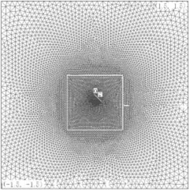
Figure 2. The domain and initial mesh.

The boundary and initial conditions (21), (24) and (25) are given by

u_{b} = 0 m / s

u_{0} = 0 m / s

, and

ω_{0} = 0 rad / s

The initial mesh has 1 7400 triangular cells. In Figure 2, the inside rectangular indicates the moving mesh zone.

5.1.1. Harmonic Vibration of the Pendulum

The object of this simulation is to compare the mesh displacements by spring networks with damping and no damping (see Eqs. (42)~(45)) and test the performance of the time adaptive method (see Eqs. (46) and (47)). The model equations for the harmonic motion in the air are Eqs. (16)~(20) neglecting the hydrodynamic moment

M_{f}

in Eq.(20). According to the algorithm mentioned above, the solution has successively performed for several periods of vibration. The time step is taken as the constant

Δt = 0.01 s

for the first 5 steps and then the adaptive step.

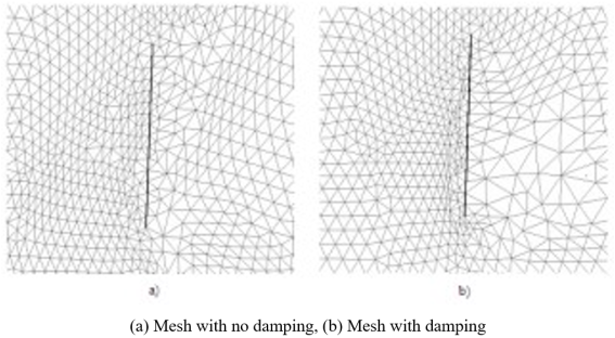
Figure 3 shows the influence of damping on the mesh displacement by the spring network at time

t = 0.165 s

. It is obvious that the state of the mesh with no damping (see the left in Figure 3) is better than one with damping (the right in Figure 3).

Download: Download full-size image

Figure 3. Influence of the damping on the mesh displacement by the spring network.

Figure 4 shows the performance of the adaptive time method. As seen in Figure 4 a, the quality of the mesh is degraded when the time step is taken as the constant step

Δt = 0.05 s

from the time

t = 0.05 s

t = 0.1 s

, though the mesh state near the rigid body is relatively good by the spring analogy method with no damping. Figure 4 b shows that when using still the constant step 0.05s, the cells with negative volume appear due to the crossing of edges, that’s, the failure of DGCL, at

t = 0.15 s

. Then, the calculation ends up incompletely.

Figure 4 c shows that the state of the mesh at time

t = 0.1 s

(see Figure 4 a)) is recovered significantly at time

t = 0.1175 s

using the adaptive time algorithm. Also, as seen in Figure 4 d, the state of the mesh is good at time

t = 0.1278 s

Download: Download full-size image

Figure 4. Effect of the adaptive time algorithm: (a) Degraded mesh for

Δt = 0.05 s

and

t = 0.1 s

, (b) Cells with negative volume for constant

Δt = 0.05 s

and

t = 0.15 s

, (c) Upgraded mesh by the adaptive algorithm from

t = 0.1 s

t = 0.1175 s

, (d) full mesh at

t = 0.1278 s

5.1.2. Damped Vibration of the Pendulum

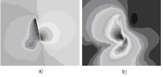
The model equations for the damped vibration of the pendulum in the air are Eqs. (16)~(20). Figure 5 shows the pressure and velocity fields at time

t = 0.184 s

when the pendulum is moving to the right. In Figure 5a, the pressure over the right overall surface of the pendulum is higher than that at the left and thus, the motion of the pendulum is damped meeting with the resistance of air. Contrarily, in Figure 5b, the velocity over the left of the pendulum is higher than that at the right. These behaviours are repeated with the damping property.

Download: Download full-size image

Figure 5. Pressure (a) and velocity (b) at time

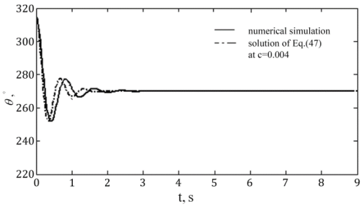
Meanwhile, the problem under consideration can be approximated by the simplest oscillator with linear viscous damping as

I \ddot{θ} + c \dot{θ} + \frac{mgl}{2} θ = 0

(48)

where

c

is the viscous damping coefficient. In the under-damped case, the viscous damping constant

c

may be determined experimentally by measuring the rate of decay of unforced oscillations.

Figure 6 shows the result by the numerical simulation (drawed by solid line in Figure 6 and the solution (dot-and-dash line) of Eq. (47) with the viscous damping

c = 0.004

. From this fact, the role of experiment for determining the viscous damping constant

c

may be replaced by the numerical simulations such as this case.

Download: Download full-size image

Figure 6. Variation of the orientation of the pendulum versus time.

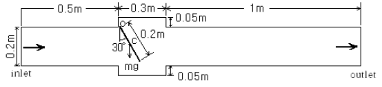
5.2. Motion and Local Resistance of a Swing Check Valve

The swing check valve is used in underwater exhaustion or fire extinguishing systems. However, the local resistance characteristics, especially when the valve is open, are determined through experiments, tests or semiempirical expression. Here, we determine the local resistance characteristics, especially when the valve is open, through the numerical simulation.

5.2.1. Numerical Simulation for the Opening Process

The air flows through the swing check valve linked by the pipe with the hydraulic diameter

d = 0.2 m

. The problem under consideration is illustrated in Figure 7. The uniform plate with mass,

m = 5 kg

and length,

l = 0.2 m

is supported by a frictionless hinge at the point O. The barycentre of the plate is the point

C

. It is open at t =0 from the angle of

θ_{0} = 30 0^{\circ}

by which the plate is displaced counter-clockwise from the horizontally right position (

x

-coordinate axis). The moment of inertia of the plate is

I = (1 / 3) m l^{2} = 0.067 kg m^{2}

and the acceleration due to gravity

g = 9.8 m / s^{2}

Download: Download full-size image

Figure 7. Schematic of the problem.

The density and viscosity of air are

ρ = 1.225 kg / m^{3}

and

μ = 1.7894 \times 1 0^{- 5} kg / ms

, respectively.

The initial conditions (24) and (25) are given by

u_{0} = 0 m / s

and

ω_{0} = 0 rad / s

. The gauge static pressures

p_{in} = 3000 Pa

and

p_{out} = 0 Pa

are given at the inlet and the outlet, respectively. The operating pressure is

p_{0} = 101325 Pa

and then the absolute pressure is the gauge static pressures plus the operating pressure. The solution has successively performed from the initial angle

θ = 30 0^{\circ} (t = 0 s)

to the full open angle

θ = 37 0^{\circ} (t = 0.18 s)

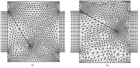
Figure 8 shows the meshes at time

t = 0 s

and

t = 0.11 s

, respectively.

Download: Download full-size image

Figure 8. Meshes at different times, (a)

t = 0 s

, (b)

t = 0.11 s

Figure 9 and Figure 10 show the total pressure fields at the intermediate time

t = 0.11 s (θ = 33 0^{\circ})

and the fully open time

t = 0.18 s (θ = 37 0^{\circ})

, respectively.

Download: Download full-size image

Figure 9. Total pressure field at the intermediate time

t = 0.11 s (θ = 33 0^{\circ})

Download: Download full-size image

Figure 10. the total pressure fields at the fully open time

t = 0.18 s (θ = 37 0^{\circ})

The average total pressure values at the inlet and the outlet of the pipe and the average velocity at the inlet at

and

are obtained as follows, respectively.

P_{in} = 2985.536 Pa, {, P}_{out} = 689.426 Pa

and

υ_{in} = 33.791 m / s

(49)

P_{in} = 2988.259 Pa, P_{out} = 2020.043 Pa

and

υ_{in} = 60.178 m / s

(50)

These values are used in the next section 5.2.2 for determining local resistence of the valve. The total pressure is defined as

P = p + \frac{1}{2} ρ υ_{in}^{2}

(51)

where

υ_{in}

is the magnitude of the velocity vector at the inlet of the pipe.

Meanwhile, suppose the pipe is the straight in the same dimensions without the valve and then, the average total pressure values at the inlet and the outlet of it and the average velocity at the inlet are obtained as follows, respectively

P_{in} = 3014.114 Pa, P_{out} = 2369.326 Pa

and

υ_{in} = 63.72 m / s

(52)

5.2.2. Local Resistance Characteristics of the Valve

The local resistance coefficient of the swing check valve can be calculated as

ξ_{v} = ξ_{t} - ξ_{s}

(53)

where

ξ_{v}

ξ_{t}

and

ξ_{s}

are the local, total and frictional resistances of the pipe system, respectively. The total resistance coefficient is calculated as

ξ_{t} = \frac{P_{in} - P_{out}}{\frac{1}{2} ρ υ_{in}^{2}}

(54)

and the frictional resistance coefficient

ξ_{s}

is also determined from Eq. (54) using Eq. (52) for the straight pipe.

Table 2 lists the values of the local resistance coefficient estimated in this way along as well as the experimental data and the semiempirical expression

[12]

ξ = 0.0845 \frac{l}{d} - 0.0053 {(\frac{l}{d})}^{2} + η (1 - \frac{1}{(1 + 0.033 \frac{l}{d})^{2}})

(55)

where

l

and

d

are the length and hydraulic diameter of the valve body, respectively and

η \approx 0.8

is the relaxation factor for the outlet part of the valve body.

Table 2. Local resistance coefficient values of the valve.

Angle Simulation Experiment Semiempirical Eq. (55)
3.025 - -
0.218 0.186 0.220

When the valve was open fully at angle

θ = 37 0^{\circ}

, the value from this simulation is in agreement with the experimental value with the error of 1%.

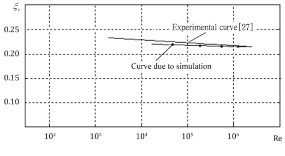
Figure 11 shows the local resistance coefficient according to Reynolds number at

θ = 37 0^{\circ}

, when the swing check valve is open fully. The Reynolds number is defined as

Re = υ_{in} d / μ

. It is seen that the discrepancy with the experimental data decreases as Reynolds number,

increases. The error with respect to the experimental data is small (<3%).

Download: Download full-size image

Figure 11. Local resistance coefficient versus Reynolds number at

θ = 37 0^{\circ}

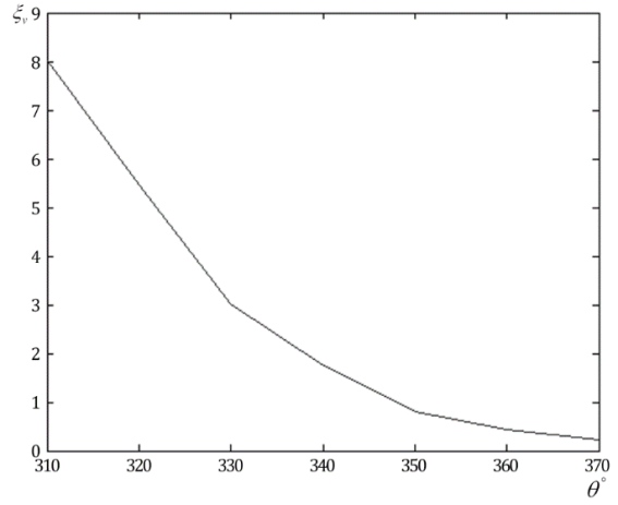
Figure 12 shows the variation of the local resistance coefficient according to the opening angle under settings mentioned above. As seen in the Figure 12, its local resistance decreases rapidly as the valve is open.

Download: Download full-size image

Figure 12. Local resistance coefficient versus the opening angle.

6. Conclusion

In the numerical method to simulate fluid and body interactions, the unique ALE formulation has presented, which includes the differential form of the geometric conservation law. Also, the adaptive time algorithm based on a Courant-Friedrichs-Levy (CFL) type condition which is estimated by the difference between the fluid and mesh velocity has presented to advance stably the numerical solutions of incompressible viscous flow past moving bodies when the motion of the bodies is not known. The numerical examples showed the ability of the adaptive time algorithm to recover the degraded mesh in combination with the method of spring smoothing with no damping. It was shown that numerical results on the damped vibration of the pendulum and the opening of the swing check valve can replace limited or impossible measurements.

Abbreviations

ALE	Arbitrary Lagrangian Eulerian

Acknowledgments

It is also the result of collaborative research with University of Sciences.

Funding

This work was partially supported by University of Sciences.

Conflicts of Interest

The authors declare no conflicts of interest.

References

[1]	Xiaodong Ren, Kun Xu, and Wei Shyy, “A multi-dimensional high-order DG-ALE method based on gas-kinetic theory with application to oscillating bodies”, Journal of Computational Physics 316, 700-720 (2016). https://doi.org/10.1016/j.jcp.2016.04.028
[2]	B. T. Helenbrook and J. Hrdina, “High-order adaptive arbitrary-Lagrangian-Eulerian (ALE) simulations of solidification”, Computers and Fluids 167, 40-50 (2018). https://doi.org/10.1016/j.compfluid.2018.02.028
[3]	P. Lonetti and R. Maletta, “Dynamic impact analysis of masonry buildings subjected to flood actions”, Engineering Structures 167, 445-458 (2018).
[4]	A. Miró, M. Soria, J. C. Cajas, and I. Rodríguez, “Numerical study of heat transfer from a synthetic impinging jet with a detailed model of the actuator membrane”, Int. J. Therm. Sci. 136, 287-298 (2019).
[5]	C. S. Peskin, “Numerical analysis of blood flow in the heart”, 220-252, J. Comput. Phys. 25(1977).
[6]	Z. Li and M. C. Lai, “Immersed interface methods for the Navier-Stokes equation with singular forces”, J. Comput. Phys. 171, 822-842 (2001).
[7]	R. Glowinski and et al., “A Fictitious Domain Approach to the Direct Numerical Simulation of Incompressible Viscous Flow past Moving Rigid Bodies: Application to Particulate Flow”, J. Comput. Phys. 169, 363-426 (2001). https://doi.org/10.1006/jcph.2000.6542
[8]	Farhat C, Geuzaine P, and Grandmont C. “The Discrete Geometric Conservation Law and the Nonlinear Stability of ALE Scheme for the Solution of Flow Problems on Moving Grids”, J. Comput. Phys. 174, 669-694 (2001).
[9]	Jeffrey Grandy, “Conservative Remapping and Region Overlays by Intersecting Arbitrary Polyhedra”, Journal of Computational Physics 148, 433-466 (1999).
[10]	P. Geuzaine, C. Grandmont, and C. Farhat, “Design and analysis of ALE schemes with provable second-order time-accuracy for inviscid and viscous flow simulations”, Journal of Computational Physics 191, 206-227 (2003). https://doi/10.1016/S0021-9991(03)00311-5
[11]	A. Hay, S. Etienne, A. Garon, and D. Pelletier, “Time-integration for ALE simulations of Fluid-Structure Interaction problems: Stepsize and order selection based on the BDF”, Comput. Methods Appl. Mech. Engrg. 295, 172-195 (2015). https://doi.org/10.1016/j.cma.2015.06.006
[12]	D. S. Kershaw, M. K. Prasad, M. J. Shaw, and J. L. Milovich, “3D unstructured mesh ALE hydrodynamics with the upwind discontinuous finite element method”, Comput. Methods Appl. Mech. Engrg. 158, 81-116 (1998).
[13]	R. T. Jung and T. Sato, “Numerical simulation of high Schmidt number flow over a droplet by using moving unstructured mesh”, J. Comput. Phys. 203, 221-249 (2005).
[14]	С. С. Золотов, “Аэродинамика судовой вентиляции”, ленин, 1975г.
[15]	Batina J, “Unsteady Euler algorithm with unstructured dynamic mesh for complex-aircraft aerodynamic analysis”, AIAA J 1991.
[16]	Jitendra Kumar Patel and Ganesh Natarajan, “Diffuse interface immersed boundary method for multi-fluid flows with arbitrarily moving rigid bodies”, J. Comput. Phys. 360, 202-228 (2018). https://doi.org/10.1016/j.jcp.2018.01.024
[17]	Chengjie Wang, Jeff D. Eldredge, et al., “Strongly coupled dynamics of fluids and rigid-body systems with the immersed boundary projection method”, Journal of Computational Physics 295, 87-113 (2015). https://doi.org/10.1016/j.jcp.2015.04.005
[18]	F. Ilinca and J. F. Hétu, “Numerical simulation of fluid-solid interaction using an immersed boundary finite element method”. Computers & Fluids 59, 31-43 (2012).
[19]	Y. Wang, C. Shu, and et al., “An immersed boundary-lattice boltzmann flux solver in a moving frame to study three-dimensional freely falling rigid bodies”, Journal of Fluids and Structures 68, 444-465 (2017). https://doi.org/10.1016/j.jfluidstructs.2016.11.005
[20]	J. Donea, “An Arbitrary Lagrangian-Eulerian finite element method for transient fluid-structure interactions”, Comput Meth Appl Mech Eng. 33, 689(1982).

Cite This Article

Plain Text BibTeX RIS

APA Style

Kim, W. I., Jo, J. W., Jo, W. H., Ri, M. C., Pyon, S. B. (2025). ALE Numerical Simulation for a Rigid Body Rotation About a Fixed Axis in a Incompressible Viscous Fluid. International Journal of Fluid Mechanics & Thermal Sciences, 11(4), 62-75. https://doi.org/10.11648/j.ijfmts.20251104.11

Copy | Download

ACS Style

Kim, W. I.; Jo, J. W.; Jo, W. H.; Ri, M. C.; Pyon, S. B. ALE Numerical Simulation for a Rigid Body Rotation About a Fixed Axis in a Incompressible Viscous Fluid. Int. J. Fluid Mech. Therm. Sci. 2025, 11(4), 62-75. doi: 10.11648/j.ijfmts.20251104.11

Copy | Download

AMA Style

Kim WI, Jo JW, Jo WH, Ri MC, Pyon SB. ALE Numerical Simulation for a Rigid Body Rotation About a Fixed Axis in a Incompressible Viscous Fluid. Int J Fluid Mech Therm Sci. 2025;11(4):62-75. doi: 10.11648/j.ijfmts.20251104.11

Copy | Download

@article{10.11648/j.ijfmts.20251104.11,
  author = {Wan Il Kim and Jae Wan Jo and Wan Hui Jo and Myong Chol Ri and Song Bom Pyon},
  title = {ALE Numerical Simulation for a Rigid Body Rotation About a Fixed Axis in a Incompressible Viscous Fluid
},
  journal = {International Journal of Fluid Mechanics & Thermal Sciences},
  volume = {11},
  number = {4},
  pages = {62-75},
  doi = {10.11648/j.ijfmts.20251104.11},
  url = {https://doi.org/10.11648/j.ijfmts.20251104.11},
  eprint = {https://article.sciencepublishinggroup.com/pdf/10.11648.j.ijfmts.20251104.11},
  abstract = {An efficient numerical method is presented in this paper. It combines a unique ALE formulation with an adaptive time algorithm based on a Courant-Friedrichs-Levy (CFL) type condition to simulate fluid and rigid body interactions. The ALE differential formulation includes the geometric conservation law (GCL) which has the mesh velocity as a variable. In the adaptive time algorithm, the time step selection is based on the CFL type condition which is estimated by the difference between the fluid and mesh velocity. With the adaptive algorithm, the numerical simulations of incompressible viscous flow around moving bodies when the motion of the bodies is not known in advance are stable. To validate the proposed method, only the body rotation about a fixed axis in a incompressible viscous fluid is considered because it causes the large deformation of mesh. The harmonic and damped vibrations of a physical pendulum in the air are tested and the opening of a swing check valve plate is simulated to determine its local resistance characteristics in comparison with experimental data. The numerical simulations show that when a rigid body rotates in an incompressible fluid, the distortion of the mesh element is not significant and the numerical results agree with the experimental data.
},
 year = {2025}
}

Copy | Download

TY  - JOUR
T1  - ALE Numerical Simulation for a Rigid Body Rotation About a Fixed Axis in a Incompressible Viscous Fluid

AU  - Wan Il Kim
AU  - Jae Wan Jo
AU  - Wan Hui Jo
AU  - Myong Chol Ri
AU  - Song Bom Pyon
Y1  - 2025/10/10
PY  - 2025
N1  - https://doi.org/10.11648/j.ijfmts.20251104.11
DO  - 10.11648/j.ijfmts.20251104.11
T2  - International Journal of Fluid Mechanics & Thermal Sciences
JF  - International Journal of Fluid Mechanics & Thermal Sciences
JO  - International Journal of Fluid Mechanics & Thermal Sciences
SP  - 62
EP  - 75
PB  - Science Publishing Group
SN  - 2469-8113
UR  - https://doi.org/10.11648/j.ijfmts.20251104.11
AB  - An efficient numerical method is presented in this paper. It combines a unique ALE formulation with an adaptive time algorithm based on a Courant-Friedrichs-Levy (CFL) type condition to simulate fluid and rigid body interactions. The ALE differential formulation includes the geometric conservation law (GCL) which has the mesh velocity as a variable. In the adaptive time algorithm, the time step selection is based on the CFL type condition which is estimated by the difference between the fluid and mesh velocity. With the adaptive algorithm, the numerical simulations of incompressible viscous flow around moving bodies when the motion of the bodies is not known in advance are stable. To validate the proposed method, only the body rotation about a fixed axis in a incompressible viscous fluid is considered because it causes the large deformation of mesh. The harmonic and damped vibrations of a physical pendulum in the air are tested and the opening of a swing check valve plate is simulated to determine its local resistance characteristics in comparison with experimental data. The numerical simulations show that when a rigid body rotates in an incompressible fluid, the distortion of the mesh element is not significant and the numerical results agree with the experimental data.

VL  - 11
IS  - 4
ER  -

Copy | Download

Author Information

Wan Il Kim

Faculty of Mechanics, Kim Chaek University of Technology, Pyongyang, DPR Korea
Jae Wan Jo

Faculty of Engineering, University of Sciences, Pyongyang, DPR Korea
Wan Hui Jo

Faculty of Engineering, University of Sciences, Pyongyang, DPR Korea
Myong Chol Ri

Faculty of Physical Engineering, Kim Chaek University of Technology, Pyongyang, DPR Korea

Contact Email

http://orcid.org/0009-0007-5835-904X
Song Bom Pyon

Faculty of Physical Engineering, Kim Chaek University of Technology, Pyongyang, DPR Korea

Download PDF

Submit an Article

Plain Text BibTeX RIS

APA Style

Kim, W. I., Jo, J. W., Jo, W. H., Ri, M. C., Pyon, S. B. (2025). ALE Numerical Simulation for a Rigid Body Rotation About a Fixed Axis in a Incompressible Viscous Fluid. International Journal of Fluid Mechanics & Thermal Sciences, 11(4), 62-75. https://doi.org/10.11648/j.ijfmts.20251104.11

Copy | Download

ACS Style

Kim, W. I.; Jo, J. W.; Jo, W. H.; Ri, M. C.; Pyon, S. B. ALE Numerical Simulation for a Rigid Body Rotation About a Fixed Axis in a Incompressible Viscous Fluid. Int. J. Fluid Mech. Therm. Sci. 2025, 11(4), 62-75. doi: 10.11648/j.ijfmts.20251104.11

Copy | Download

AMA Style

Kim WI, Jo JW, Jo WH, Ri MC, Pyon SB. ALE Numerical Simulation for a Rigid Body Rotation About a Fixed Axis in a Incompressible Viscous Fluid. Int J Fluid Mech Therm Sci. 2025;11(4):62-75. doi: 10.11648/j.ijfmts.20251104.11

Copy | Download

@article{10.11648/j.ijfmts.20251104.11,
  author = {Wan Il Kim and Jae Wan Jo and Wan Hui Jo and Myong Chol Ri and Song Bom Pyon},
  title = {ALE Numerical Simulation for a Rigid Body Rotation About a Fixed Axis in a Incompressible Viscous Fluid
},
  journal = {International Journal of Fluid Mechanics & Thermal Sciences},
  volume = {11},
  number = {4},
  pages = {62-75},
  doi = {10.11648/j.ijfmts.20251104.11},
  url = {https://doi.org/10.11648/j.ijfmts.20251104.11},
  eprint = {https://article.sciencepublishinggroup.com/pdf/10.11648.j.ijfmts.20251104.11},
  abstract = {An efficient numerical method is presented in this paper. It combines a unique ALE formulation with an adaptive time algorithm based on a Courant-Friedrichs-Levy (CFL) type condition to simulate fluid and rigid body interactions. The ALE differential formulation includes the geometric conservation law (GCL) which has the mesh velocity as a variable. In the adaptive time algorithm, the time step selection is based on the CFL type condition which is estimated by the difference between the fluid and mesh velocity. With the adaptive algorithm, the numerical simulations of incompressible viscous flow around moving bodies when the motion of the bodies is not known in advance are stable. To validate the proposed method, only the body rotation about a fixed axis in a incompressible viscous fluid is considered because it causes the large deformation of mesh. The harmonic and damped vibrations of a physical pendulum in the air are tested and the opening of a swing check valve plate is simulated to determine its local resistance characteristics in comparison with experimental data. The numerical simulations show that when a rigid body rotates in an incompressible fluid, the distortion of the mesh element is not significant and the numerical results agree with the experimental data.
},
 year = {2025}
}

Copy | Download

TY  - JOUR
T1  - ALE Numerical Simulation for a Rigid Body Rotation About a Fixed Axis in a Incompressible Viscous Fluid

AU  - Wan Il Kim
AU  - Jae Wan Jo
AU  - Wan Hui Jo
AU  - Myong Chol Ri
AU  - Song Bom Pyon
Y1  - 2025/10/10
PY  - 2025
N1  - https://doi.org/10.11648/j.ijfmts.20251104.11
DO  - 10.11648/j.ijfmts.20251104.11
T2  - International Journal of Fluid Mechanics & Thermal Sciences
JF  - International Journal of Fluid Mechanics & Thermal Sciences
JO  - International Journal of Fluid Mechanics & Thermal Sciences
SP  - 62
EP  - 75
PB  - Science Publishing Group
SN  - 2469-8113
UR  - https://doi.org/10.11648/j.ijfmts.20251104.11
AB  - An efficient numerical method is presented in this paper. It combines a unique ALE formulation with an adaptive time algorithm based on a Courant-Friedrichs-Levy (CFL) type condition to simulate fluid and rigid body interactions. The ALE differential formulation includes the geometric conservation law (GCL) which has the mesh velocity as a variable. In the adaptive time algorithm, the time step selection is based on the CFL type condition which is estimated by the difference between the fluid and mesh velocity. With the adaptive algorithm, the numerical simulations of incompressible viscous flow around moving bodies when the motion of the bodies is not known in advance are stable. To validate the proposed method, only the body rotation about a fixed axis in a incompressible viscous fluid is considered because it causes the large deformation of mesh. The harmonic and damped vibrations of a physical pendulum in the air are tested and the opening of a swing check valve plate is simulated to determine its local resistance characteristics in comparison with experimental data. The numerical simulations show that when a rigid body rotates in an incompressible fluid, the distortion of the mesh element is not significant and the numerical results agree with the experimental data.

VL  - 11
IS  - 4
ER  -

Copy | Download