Confidence-Weighted Multiscale Point-to-Plane Change Detection for Point-Cloud-Based Object Monitoring

Yaxshibayev Doniyor Sultonbayevich; Kudratov Sultan Gulamovich; Rakhmatov Furkat Abdurazzokovich

doi:doi:10.11648/j.mcs.20261105.12

Research Article |

| Peer-Reviewed

Confidence-Weighted Multiscale Point-to-Plane Change Detection for Point-Cloud-Based Object Monitoring

Yaxshibayev Doniyor Sultonbayevich

, Kudratov Sultan Gulamovich^*

, Rakhmatov Furkat Abdurazzokovich

Published in Mathematics and Computer Science (Volume 11, Issue 5)

Received: 7 September 2026 Accepted: 17 September 2026 Published: 30 September 2026

Views: Downloads:

Download PDF

Share This Article

Twitter
Linked In
Facebook

Abstract

Repeated three-dimensional point clouds provide a practical basis for monitoring local geometric deformation, but conventional pointwise or single-scale comparison is sensitive to residual registration error, nonuniform sampling, measurement noise, missing observations, and isolated outliers. To address these limitations, this study develops an interpretable confidence-weighted multiscale point-to-plane detector for spatially coherent change in repeated point clouds. Local normals are estimated from covariance matrices at several neighbourhood scales; point-to-plane residuals are fused across scales, modulated by a planarity-density confidence term, thresholded with the median absolute deviation (MAD), and filtered by neighbourhood persistence. The MATLAB implementation was evaluated on a controlled non-planar synthetic surface with Gaussian deformation, rigid displacement, heterogeneous noise, nonuniform sampling, dropout, and outliers. Across 30 independent Monte Carlo realisations, the complete method achieved precision 0.836 ± 0.030, recall 0.967 ± 0.012, F1 0.897 ± 0.018, IoU 0.813 ± 0.029, and FPR 0.0071 ± 0.0018. The single-scale point-to-plane baseline reached F1 0.625 ± 0.021, while confidence-weighted multiscale scoring without persistence reached 0.640 ± 0.019. Trimmed ICP reduced robust nearest-neighbour RMSE from 7.262 ± 0.032 mm to 0.771 ± 0.009 mm. Across tested deformation amplitudes from 3 to 10 mm, F1 increased from 0.749 to 0.930. The results show that spatial persistence provides the largest improvement in false-alarm suppression, with confidence weighting adding a complementary gain. All results are synthetic; sensor-specific detection limits and field accuracy are not claimed.

Published in	Mathematics and Computer Science (Volume 11, Issue 5)
DOI	10.11648/j.mcs.20261105.12
Page(s)	106-117
Creative Commons	This is an Open Access article, distributed under the terms of the Creative Commons Attribution 4.0 International License (http://creativecommons.org/licenses/by/4.0/), which permits unrestricted use, distribution and reproduction in any medium or format, provided the original work is properly cited.
Copyright	Copyright © The Author(s), 2026. Published by Science Publishing Group

Keywords

3D Monitoring, Deformation Detection, Geometric Residual, Multiscale Analysis, Point-Cloud Registration, Spatial Persistence

1. Introduction

Repeated 3D point clouds are increasingly used to detect geometric changes in structural surfaces, industrial components, terrain, façades, and other monitored objects. The underlying task is deceptively simple: align two observations and identify regions that have changed. In practice, however, two scans of an unchanged surface are not identical. Their samples occupy different positions, point density varies spatially, occlusion changes the visible surface, and the measurements contain sensor noise and occasional outliers. These acquisition effects can produce nonzero point-to-point distances without any physical deformation.

Rigid registration is commonly performed using the iterative closest point (ICP) family

[1, 2]

, its point-to-plane variants

[3]

, efficient refinements

[4]

, or probabilistic approaches such as coherent point drift (CPD)

[5]

. Registration is necessary but not sufficient for monitoring. A transformation may minimise the global distance between two point sets while local residuals still contain contributions from sampling geometry, registration uncertainty, measurement noise, and true deformation. A change detector must therefore treat global alignment and local change inference as related but distinct stages.

Direct Euclidean nearest-neighbour distance is especially sensitive to tangential resampling. On a smooth surface, two independently sampled points may be separated tangentially although their underlying surfaces coincide. Projecting the local discrepancy onto an estimated surface normal reduces this ambiguity. Surface-normal estimation from local covariance analysis is a standard geometric construction for unorganised point sets

[6]

. Multiscale neighbourhood analysis is also useful because normal stability and geometric detail depend on the physical support used for estimation

[7, 8]

. In point-cloud change detection, multiscale surface comparison has been shown to improve robustness in complex natural geometry

[9, 10]

Recent point-cloud change-analysis research has also moved toward spatiotemporal segmentation and learning-based detectors. The 4D Objects-By-Change framework treats persistent 3D surface changes as spatiotemporal objects

[12]

, while Siamese KPConv learns multiple change classes directly from paired raw point clouds

[13]

. In parallel, modern registration approaches such as GeoTransformer and PointDSC improve correspondence robustness under difficult overlap and outlier conditions

[14, 15]

. Recent 2024 studies further extend this literature: change-aware deep networks improve direct change segmentation in raw 3D point clouds

[16]

, while engineering monitoring studies use terrestrial laser scanning with ICP-based multi-epoch deformation analysis for earth dams

[17]

and sliding-window surface fitting for bridge deformation

[18]

. These advances are complementary to the present study: our objective is not semantic change classification or learned feature matching, but an interpretable geometric detector whose individual stages can be inspected and calibrated.

A further difficulty is threshold selection. A single absolute distance threshold is difficult to justify when sampling and noise vary across the object. Robust scale estimators based on the median absolute deviation (MAD) offer a data-dependent alternative that is less sensitive to a minority of large residuals than a mean-and-standard-deviation rule

[11]

. Even with a robust threshold, isolated correspondence errors or outliers can remain. For many monitoring tasks, a physically meaningful surface deformation is expected to influence a spatial neighbourhood rather than a single sample. This motivates a second decision stage based on spatial persistence.

The aim of this study is to formulate and evaluate a confidence-weighted multiscale point-to-plane detector for repeated point clouds. The proposed method has four components: (1) point-to-plane residuals evaluated at several neighbourhood scales; (2) a local geometric-confidence factor combining planarity and a normalised neighbourhood-density proxy; (3) a robust MAD-based threshold; and (4) a neighbourhood-persistence rule for suppressing isolated responses. The entire processing chain is implemented in MATLAB and demonstrated on a controlled synthetic surface with known local deformation.

The combination of the four components is deliberate. Multiscale fusion reduces dependence on a single neighbourhood support, confidence weighting attenuates geometrically unstable estimates, and spatial persistence suppresses isolated threshold exceedances. None of these ingredients is claimed as novel in isolation; the methodological contribution is their integrated, quantitatively ablated use for repeated point-cloud monitoring under a controlled error model.

The contribution is methodological rather than metrological. In addition to the representative score and decision maps, the controlled experiment includes repeated Monte Carlo comparison, component ablation, registration diagnostics, robustness sweeps, parameter sensitivity, and deformation-amplitude analysis. These tests quantify algorithmic behaviour under known synthetic ground truth but do not establish a minimum detectable deformation for a particular laser scanner, camera, or photogrammetric system. Such claims require repeated physical measurements and independent displacement ground truth.

2. Materials and Methods

2.1. Repeated Point-Cloud Model

Let the reference point cloud acquired at time

t_{0}

P = {p_{i} \in R^{3}}_{i = 1}^{N}

and the monitoring cloud acquired at time

t_{1}

Q = {q_{j} \in R^{3}}_{j = 1}^{M}

. A monitoring observation is modelled conceptually as

q = R [p + d (p)] + t + ε,

(1)

where

R \in SO (3)

and

t \in R^{3}

describe the rigid transformation between coordinate systems,

d (p)

is the physical deformation field, and

ε

denotes acquisition error. A rigid transformation is first estimated and applied to

Q

so that subsequent change analysis is performed in the reference coordinate system. The alignment stage follows the nearest-neighbour ICP principle

[1, 2, 4]

; the monitoring decision is computed only after registration.

2.2. Local Surface Geometry

For each reference point

p_{i}

and scale

s

, let

N_{i}^{(s)}

contain

k_{s}

nearest neighbours. The local centroid is

μ_{i}^{(s)} = \frac{1}{k_{s}} \sum_{p_{j} \in N_{i}^{(s)}} p_{j},

(2)

and the local covariance matrix is

C_{i}^{(s)} = \frac{1}{k_{s} - 1} \sum_{p_{j} \in N_{i}^{(s)}} (p_{j} - μ_{i}^{(s)}) {(p_{j} - μ_{i}^{(s)})}^{T}

(3)

Let the eigenvalues of

C_{i}^{(s)}

satisfy

λ_{1, i}^{(s)} \geq λ_{2, i}^{(s)} \geq λ_{3, i}^{(s)} \geq 0

. The eigenvector corresponding to

λ_{3, i}^{(s)}

is taken as the local surface normal

n_{i}^{(s)}

[6]

. A planarity-related confidence component is defined as

g_{i}^{(s)} = \frac{λ_{2, i}^{(s)} - λ_{3, i}^{(s)}}{λ_{1, i}^{(s)} + ϵ_{λ}}, ϵ_{λ} > 0 .

(4)

The positive numerical stabilisers used in Equations (4)-(6) are denominator-specific safeguards. They are distinguished in the analytical notation so that each has the physical dimension of the denominator in which it appears; in the MATLAB implementation the corresponding machine-precision safeguard is represented by eps because all quantities are evaluated numerically in SI units.

2.3. Neighbourhood-Density Proxy and Geometric Confidence

The implementation uses a three-dimensional

k

-nearest-neighbour density proxy based on the radius

r_{i, k_{s}}

to the

k_{s}

-th neighbour:

{\tilde{ρ}}_{i}^{(s)} = \frac{k_{s}}{\frac{4}{3} π r_{i, k_{s}}^{3} + ϵ_{V}} .

(5)

Equation (5) is not interpreted as the physical areal density of samples on a surface. It is a volumetric neighbourhood-density proxy in the ambient 3D coordinate space. Because only its dimensionless normalised ratio is used in the final confidence term, its purpose is to identify locally sparse neighbourhoods while preserving the MATLAB implementation that generated the reported figures. An areal proxy proportional to

r^{- 2}

would define a different weighting model and would require re-running the experiment before replacing Equation (5).

On strongly curved surfaces, a spherical 3D neighbourhood can contain points that are close in Euclidean distance but poorly representative of the local tangent patch, which may bias this proxy. A future areal alternative could estimate density after projection onto the local tangent plane or from a locally reconstructed surface patch; such a replacement would require recalibration and a new experimental evaluation.

The normalised density factor is

d_{i}^{(s)} = \min [1, \frac{{\tilde{ρ}}_{i}^{(s)}}{{median}_{j} ({\tilde{ρ}}_{j}^{(s)}) + ϵ_{ρ}}],

(6)

and the geometric confidence is

c_{i}^{(s)} = \min [1, \max (c_{\min}, g_{i}^{(s)} d_{i}^{(s)})] .

(7)

The lower bound

c_{\min}

prevents a valid but sparsely sampled region from being completely suppressed. In the reported simulation,

c_{\min} = 0.05

2.4. Confidence-Weighted Multiscale Change Score

After registration,

q_{ν (i)}

denotes the monitoring point assigned by nearest-neighbour association to

p_{i}

. At scale

s

, the signed point-to-plane residual and its magnitude are

e_{i}^{(s)} = {(n_{i}^{(s)})}^{T} (q_{ν (i)} - p_{i}), r_{i}^{(s)} = |e_{i}^{(s)}| .

(8)

The simulation uses

S = 3

neighbourhood sizes,

k_{s} \in {10, 20, 40}

. The multiscale residual and mean confidence are

{\bar{r}}_{i} = \frac{1}{S} \sum_{s = 1}^{S} r_{i}^{(s)}, {\bar{c}}_{i} = \frac{1}{S} \sum_{s = 1}^{S} c_{i}^{(s)} .

(9)

The continuous change score is

z_{i} = {\bar{r}}_{i} {({\bar{c}}_{i})}^{β}, 0 \leq β \leq 1 .

(10)

A small exponent is used so that confidence attenuates geometrically unstable observations without removing them. The reported simulation uses

β = 0.10

The nearest-neighbour association used here is intentionally simple and can be ambiguous on repetitive geometry, thin structures, sharp edges, or under large tangential displacement. More restrictive schemes can impose normal compatibility, bidirectional consistency, local descriptors, or probabilistic matching, but these add computational and modelling complexity and would alter the residual error model.

2.5. Robust Threshold and Spatial Persistence

Let

m_{z} = {median}_{i} (z_{i})

and

{MAD}_{z} = {median}_{i} |z_{i} - m_{z}|

. The robust scale estimate follows the normal-consistency scaling of the MAD

[11]

σ_{z}^{*} = 1.4826 {MAD}_{z}, T = m_{z} + γ σ_{z}^{*} .

(11)

Candidate points satisfy

z_{i} > T

. For each candidate, let

M_{i}

contain its

K

nearest reference neighbours. The neighbourhood-support ratio is

h_{i} = \frac{1}{K} \sum_{j \in M_{i}} I (z_{j} > T),

(12)

where

I (\cdot)

is the indicator function. The final decision is

{\hat{y}}_{i} = \{\begin{matrix} 1, & z_{i} > T and h_{i} \geq η, \\ 0, & otherwise . \end{matrix}

(13)

This rule encodes the assumption that the target deformation is spatially coherent. It should not be applied without calibration to defects whose footprint approaches the local point spacing.

In particular, narrow cracks, small impact damage, or other genuine defects whose footprint is smaller than the persistence neighbourhood can be rejected despite a high local score. The persistence settings must therefore be calibrated against the minimum spatial footprint of defects that are relevant to the intended application.

2.6. Synthetic Surface and Deformation Model

A non-planar reference surface was generated over

0 \leq x \leq 1 m

and

0 \leq y \leq 0.6 m

. Define the dimensionless coordinates

u = x / (1 m)

and

v = y / (0.6 m)

. The same surface used in the MATLAB implementation can then be written in a dimensionally explicit and compact form as

z (u, v) = 0.018 m sin (2 πu) \sin (2 πv) + 0.0024 m uv

(14)

The local deformation field is Gaussian:

δ (x, y) = A \exp ​ [- \frac{1}{2} {(\frac{x - x_{c}}{σ_{x}})}^{2} - \frac{1}{2} {(\frac{y - y_{c}}{σ_{y}})}^{2}] .

(15)

A reference point is labelled as changed in the synthetic ground truth when

y_{i} = I ​ [δ (x_{i}, y_{i}) > 0.002 m] .

(16)

Equation (16) defines the point-level ground truth used when quantitative classification metrics are exported from a MATLAB run.

2.7. MATLAB Implementation and Reproducibility Parameters

The nominal parameters in Table 1 reproduce the MATLAB implementation used for the representative visualisation (seed 42). For quantitative comparison and ablation, the complete stochastic generation and processing chain was repeated for 30 independent random seeds. Robustness, parameter-sensitivity, and deformation-amplitude sweeps used 15 independent realisations per setting. Within each seed, all compared methods processed the same generated reference and monitoring clouds, so differences are attributable to the detector configuration rather than to different random inputs. The registration stage used the same trimmed nearest-neighbour ICP settings in every configuration.

Table 1. Main parameters of the MATLAB simulation and processing workflow.

Parameter	Value	Meaning
$N$	7000	Number of reference points
Random seed	42	Reproducible stochastic realisation
$A$	$0.006 m$	Maximum local deformation
$(x_{c}, y_{c})$	$(0.67, 0.32) m$	Deformation centre
$(σ_{x}, σ_{y})$	$(0.07, 0.055) m$	Deformation spread
Ground-truth threshold	$0.002 m$	Changed-point label in Equation (16)
Reference noise	$0.25 / 0.70 mm$	Heterogeneous Gaussian noise
Monitoring noise	$0.35 / 1.00 mm$	Heterogeneous Gaussian noise
Dropout probability	$0.12 / 0.32$	Missing monitoring points
Outlier fraction	$1 %$	Uniform isolated outliers
Rotation	${(0.45, - 0.35, 0.30)}^{\circ}$	Rigid coordinate displacement
Translation	$(4, - 3, 2) mm$	Rigid coordinate displacement
Dense-sampling fraction	$0.25$	Nonuniform sampling perturbation
Dense-region $x$ distribution	$Beta (2, 5)$	Additional sampling-density variation
ICP trimming fraction	$0.85$	Fraction retained in each alignment iteration
ICP maximum iterations	60	Registration stopping bound
ICP convergence tolerance	$10^{- 8} m$	RMSE-change criterion
$k_{s}$	${10, 20, 40}$	Normal-estimation neighbourhoods
$c_{\min}$	$0.05$	Confidence lower bound
$β$	$0.10$	Confidence exponent
$γ$	$3.5$	MAD threshold coefficient
$K$	15	Persistence neighbourhood
$η$	$0.35$	Minimum support ratio

In Table 1, paired noise and dropout values refer respectively to the general region and the higher-noise subregion

x > 0.78 m

. The synthetic sampling includes a denser region generated by replacing the

x

coordinate of

25 %

of points with samples from a

Beta (2, 5)

distribution. This deliberately breaks spatial uniformity. The high-noise and high-dropout subregion for

x > 0.78 m

provides an additional stress test for the confidence term and edge behaviour.

For practical calibration, the persistence neighbourhood K should be chosen so that its physical support radius does not substantially exceed the minimum defect footprint of interest, while eta should represent the minimum expected fraction of locally consistent detections. If point density varies strongly, a radius-based persistence neighbourhood may be preferable to a fixed neighbour count. The sensitivity results in Section 4.6 show that eta and K materially affect F1; the reported sweeps are used as calibration evidence rather than as test-set optimisation.

2.8. Evaluation Criteria and Ablation Protocol

When the binary ground truth from Equation (16) is available, the detector can be quantified using precision, recall, F1 score, intersection over union (IoU), and false-positive rate (FPR):

Precision = \frac{TP}{TP + FP}, Recall = \frac{TP}{TP + FN},

(17)

F_{1} = \frac{2 Precision Recall}{Precision + Recall}, IoU = \frac{TP}{TP + FP + FN},

(18)

FPR = \frac{FP}{FP + TN} .

(19)

Two complementary comparisons were performed on identical input clouds. The baseline comparison used five configurations: (A) Euclidean nearest-neighbour distance; (B) single-scale point-to-plane residual with

k = 20

; (C) unweighted multiscale point-to-plane residuals with

k \in {10, 20, 40}

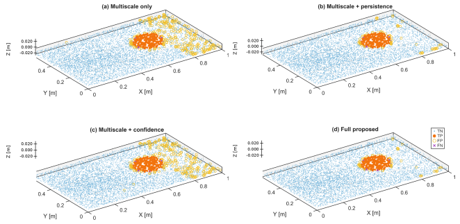
; (D) confidence-weighted multiscale scoring without persistence; and (E) the complete method. A focused four-way ablation, reported in Table 3 and visualised in Figure 3, used: multiscale only, multiscale plus spatial persistence, multiscale plus confidence, and the full proposed method. Together these comparisons isolate the effects of normal projection, multiscale fusion, confidence weighting, and spatial persistence.

For each run, the validation workflow records TP, FP, FN, TN and the derived classification metrics. The method-comparison and ablation results in Tables 2 and 3 are reported as mean ± standard deviation over 30 independent realisations, while the robustness, parameter-sensitivity, and deformation-amplitude sweeps use 15 realisations per setting. The supplementary MATLAB script supplied with this revision reproduces the representative seed-42 processing chain, Figures 1-3, and the seed-42 ablation CSV; it is not presented as the multi-seed driver for the aggregate statistics. The broader validation workflow underlying the 30-run and 15-run summaries can be supplied by the corresponding author. Because the changed region occupies only a small fraction of the cloud, the discussion emphasises precision, recall, F1, IoU, and FPR rather than overall accuracy.

3. Results

3.1. Multiscale Change-Score Distribution

Download: Download full-size image

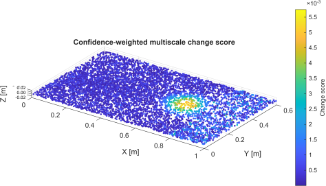
Figure 1. Confidence-weighted multiscale change score for the representative synthetic realisation (seed 42).

Figure 1 shows the continuous score

z_{i}

over the complete simulated surface. Most points remain in the low-response range, while a compact region of elevated values is concentrated around

x \approx 0.65

0.75 m

and

y \approx 0.25

0.35 m

. This location is consistent with the imposed deformation centre

(x_{c}, y_{c}) = (0.67, 0.32) m

. The colour scale reaches approximately

5.5 \times 10^{- 3}

in the highest-response zone. The transition from the background to the deformation core is spatially gradual rather than randomly scattered, which is consistent with the Gaussian deformation field and the neighbourhood-based construction of the score.

The nonzero background is expected. The monitoring cloud differs from the reference cloud not only by the prescribed deformation but also by heterogeneous noise, nonuniform density, dropout, outliers, and residual registration error. The relevant result is therefore the contrast between the spatially diffuse background and the compact high-score region, rather than an expectation of zero residual outside the changed area.

3.2. Final Deformation Map

Download: Download full-size image

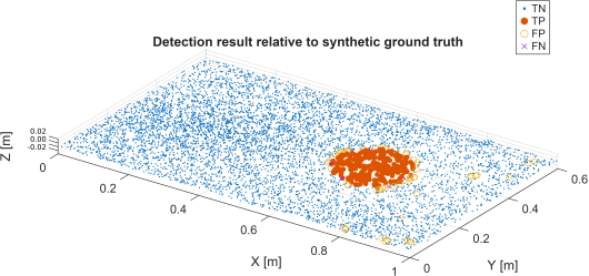
Figure 2. Detected deformation region after robust thresholding and spatial-persistence filtering (seed 42). Legend: TN, true negative; TP, true positive; FP, false positive; FN, false negative.

Figure 2 presents the final binary decision after MAD thresholding and neighbourhood-persistence filtering. The detected points form a dense, spatially coherent cluster in the same region that produces the highest continuous scores in Figure 1. This agreement between the score field and the binary map is important for interpretation: the final detector is responding primarily to a connected geometric pattern rather than to a uniformly scattered set of large residuals.

A limited number of isolated detections remain outside the main region, particularly near the sampled-surface boundaries. In the synthetic experiment these responses cannot represent additional physical defects because only one deformation field was prescribed. They are therefore attributable to the combined effects of local correspondence ambiguity, sparse neighbourhoods, outliers, noise, and residual alignment error. Their presence illustrates why a monitoring decision should be interpreted together with the continuous score and local confidence, rather than from the binary map alone.

3.3. Quantitative Comparison and Ablation

Across 30 independent Monte Carlo realisations, the complete detector achieved precision 0.836 ± 0.030, recall 0.967 ± 0.012, F1 0.897 ± 0.018, IoU 0.813 ± 0.029, and FPR 0.0071 ± 0.0018 (Table 2). The point-to-point baseline was dominated by false positives (precision 0.156; FPR 0.147), while the single-scale point-to-plane baseline raised F1 to 0.625. Unweighted multiscale fusion was nearly identical (F1 0.625), and confidence weighting without spatial persistence increased F1 modestly to 0.640. Thus, the full method improved F1 by 0.272 over the single-scale point-to-plane baseline while reducing FPR from 0.0418 to 0.0071.

Table 2. Baseline comparison over 30 Monte Carlo realisations (mean ± SD).

Method	Precision	Recall	F1	IoU	FPR
P2P NN	0.156 ± 0.012	0.734 ± 0.039	0.257 ± 0.017	0.147 ± 0.011	0.1474 ± 0.0040
P2Plane k=20	0.462 ± 0.022	0.969 ± 0.012	0.625 ± 0.021	0.455 ± 0.022	0.0418 ± 0.0023
Multiscale	0.462 ± 0.023	0.969 ± 0.011	0.625 ± 0.021	0.455 ± 0.023	0.0417 ± 0.0024
MS + confidence	0.478 ± 0.021	0.968 ± 0.012	0.640 ± 0.019	0.471 ± 0.021	0.0391 ± 0.0025
Proposed	0.836 ± 0.030	0.967 ± 0.012	0.897 ± 0.018	0.813 ± 0.029	0.0071 ± 0.0018

Ablation results isolate the source of this gain (Table 3). Adding spatial persistence to the unweighted multiscale detector increased F1 from 0.625 to 0.885 and reduced FPR from 0.0417 to 0.00816 while leaving recall essentially unchanged (0.969 to 0.969). Adding confidence weighting on top of persistence further increased precision from 0.815 to 0.836, F1 from 0.885 to 0.897, and IoU from 0.794 to 0.813. Spatial persistence therefore provides the dominant false-alarm suppression in this synthetic benchmark, whereas confidence weighting adds a smaller complementary improvement. Representative seed-42 detection maps for the four Table 3 configurations are shown in Figure 3.

Table 3. Ablation of confidence weighting and spatial persistence (mean ± SD, n = 30).

Configuration	Precision	F1	IoU	FPR
Multiscale only	0.462 ± 0.023	0.625 ± 0.021	0.455 ± 0.023	0.0417 ± 0.0024
MS + persistence	0.815 ± 0.028	0.885 ± 0.018	0.794 ± 0.029	0.0082 ± 0.0016
MS + confidence	0.478 ± 0.021	0.640 ± 0.019	0.471 ± 0.021	0.0391 ± 0.0025
Full proposed	0.836 ± 0.030	0.897 ± 0.018	0.813 ± 0.029	0.0071 ± 0.0018

Download: Download full-size image

Figure 3. Representative visual ablation maps for the synthetic realisation (seed 42): (a) unweighted multiscale point-to-plane detection; (b) multiscale detection with spatial persistence; (c) confidence-weighted multiscale detection without persistence; and (d) the complete proposed method. TN, TP, FP, and FN denote true negatives, true positives, false positives, and false negatives relative to the known synthetic ground truth, respectively.

Figure 3 provides a visual counterpart to the quantitative ablation results in Table 3. The unweighted multiscale detector produces numerous spatially scattered false-positive responses outside the imposed deformation region. Adding spatial persistence removes most isolated responses while preserving the principal changed area. Confidence weighting alone produces a more modest reduction in unstable detections, consistent with the numerical ablation results. The complete method combines both mechanisms and yields the most spatially coherent detection pattern with substantially fewer false positives. The figure corresponds to the representative seed-42 synthetic realisation; the statistics reported in Table 3 remain the mean ± standard deviation over 30 independent realisations.

Registration diagnostics showed that trimmed ICP reduced robust nearest-neighbour RMSE from 7.262 ± 0.032 mm before alignment to 0.771 ± 0.009 mm after alignment, an 89.38 ± 0.10% reduction. In 15-run amplitude sweeps, mean F1 increased from 0.749 at 3 mm to 0.839, 0.871, 0.894, 0.916, and 0.930 at 4, 5, 6, 8, and 10 mm, respectively. The 3-10 mm sweep represents millimetre-scale, spatially coherent local deflection or dent-like change under the present synthetic geometry. It is a sensitivity study, not a sensor-specific detection limit, and the reported performance must not be transferred directly to sub-millimetre deformation tasks. Outlier fractions from 0 to 5% produced F1 values between 0.893 and 0.905, while doubling the nominal dropout reduced F1 to 0.854. The measurement-noise sweep was non-monotonic: F1 was 0.727 at 0.5× noise, 0.893 at nominal noise, 0.806 at 1.5×, and 0.640 at 2×, reflecting interaction between the adaptive MAD threshold and the score distribution.

4. Discussion

4.1. Geometric Interpretation of Point-to-Plane Residuals

The observed behaviour supports the geometric rationale of the point-to-plane residual. Euclidean nearest-neighbour separation contains both normal and tangential components. When two point clouds sample the same continuous surface at different locations, the tangential component can be nonzero despite the absence of physical motion. Point-to-plane comparison, introduced widely in registration and surface comparison

[3, 9, 10]

, reduces this particular ambiguity by retaining the local normal component.

This advantage depends on the quality of the estimated normal. Local covariance analysis

[6]

is stable only when the neighbourhood contains enough geometrically informative points. On sharp edges, high curvature, or sparse sampling, a single planar normal can be a poor approximation. The proposed confidence term is intended to identify part of this instability rather than to certify metrological accuracy.

4.2. Role of Scale and Confidence

The neighbourhood set

{10, 20, 40}

should be interpreted as a discrete approximation to several support sizes rather than as an intrinsic property of the monitored object. Small neighbourhoods preserve local detail but are more sensitive to noise; larger neighbourhoods stabilise local orientation but can smooth small defects. This scale dependence is a general property of point-sampled surface analysis

[7, 8]

Neighbour count and physical support radius are not equivalent. In a dense region,

k = 40

may span only a small area, whereas the same

k

can cover a much larger patch in a sparse region. The normalised density proxy in Equations (5)-(7) therefore provides context for the reliability of the covariance estimate. Because Equation (5) uses a 3D spherical proxy, it should not be interpreted as an estimator of surface sampling density in points per square metre. If a future version replaces it with an areal density model, the MATLAB experiment must be repeated and the figures regenerated.

Curvature introduces a second source of reduced confidence. A large neighbourhood on a curved surface may violate the local-planarity assumption and produce an averaged normal. Low confidence can therefore reflect sparse sampling, complex geometry, or both. During field interpretation, these causes should be distinguished rather than treating every low-confidence point as a measurement failure.

4.3. Spatial Persistence and Alarm Reliability

Spatial persistence encodes information that is absent from a pointwise residual. The ablation results quantify its effect: applying persistence to the unweighted multiscale score increased precision from 0.462 to 0.815 and F1 from 0.625 to 0.885, while reducing FPR by approximately 80% (0.0417 to 0.00816) with essentially unchanged recall. This confirms that, for the present spatially coherent Gaussian deformation, neighbourhood support primarily removes isolated false responses rather than suppressing true changed points.

The same mechanism creates a limitation. If the support neighbourhood

K

spans a physical region wider than a narrow crack or local impact, a true change may fail the support condition even when its local score is high. Conversely, a very small

K

provides little protection against clustered outliers. The pair

(K, η)

must therefore be calibrated against local point spacing and the minimum spatial footprint of a relevant defect. Reporting

K

only as a number of points is insufficient when point density varies strongly across datasets.

4.4. Robust Thresholding and Failure Modes

The global MAD threshold is robust to a minority of large residuals

[11]

, but it assumes that unchanged points dominate the score distribution. If a large fraction of the monitored object changes, the changed population can contaminate the background estimate. Regional thresholds, stable reference zones, or mixture models may then be preferable.

A second failure mode is a spatially structured registration error. A small residual rotation or translation can create a smooth score gradient over a large part of the object. Such a pattern may satisfy the persistence condition even though it is not physical deformation. Registration quality must therefore be assessed independently before change classification. Useful diagnostics include the residual distribution in known stable regions, repeated registration from different initial conditions, and comparison with external control measurements when available.

Nearest-neighbour association is also an approximation. It can become ambiguous on repetitive geometry, thin structures, sharp edges, or surfaces with large tangential motion. More restrictive correspondence rules could incorporate normal compatibility, bidirectional consistency, local descriptors, or probabilistic matching

[5]

. Any such change alters the error model and should be evaluated independently rather than assumed to improve performance automatically.

4.5. Uncertainty and Traceability

The score

z_{i}

is influenced by sensor noise, local point spacing, registration uncertainty, normal-estimation error, correspondence ambiguity, dropout, and outliers. The current confidence coefficient represents only local geometric reliability; it is not a formal probability or a complete uncertainty interval. A high value of

c_{i}^{(s)}

therefore indicates a locally stable surface estimate under the adopted model, not guaranteed accuracy of the full measurement chain.

Traceability requires each result to be linked to a documented set of inputs and parameters. A minimal run record should contain source point-cloud identifiers, coordinate units, preprocessing operations, random seed, registration settings, neighbourhood scales,

c_{\min}

β

γ

K

η

, and the software version. The stored outputs should include the rigid transformation, continuous score vector, threshold value, candidate mask, persistence values, and final labels. This allows an engineer or reviewer to reproduce why a particular point was classified as changed.

Negative and positive controls are equally important. Repeated scans of an unchanged object estimate the false-alarm behaviour under realistic acquisition variation. A controlled deformation with an independently measured displacement verifies that the method can recover a change of practical relevance. These controls provide a more defensible basis for threshold selection than tuning the detector on a single synthetic example.

4.6. Robustness and Parameter Sensitivity

The robustness sweeps indicate that different disturbance mechanisms affect the detector differently. Outlier contamination from 0 to 5% had little effect on mean F1 (0.893-0.905), consistent with trimmed registration, MAD thresholding, and persistence rejecting isolated responses. Increasing dropout produced a gradual decline from F1 0.908 at half the nominal dropout to 0.854 at twice the nominal level, mainly through reduced precision. These results support robustness to moderate point loss and isolated outliers within the tested synthetic ranges.

The noise sweep requires a more cautious interpretation. Mean F1 was 0.727 at 0.5×, 0.893 at 1×, 0.806 at 1.5×, and 0.640 at 2× the nominal measurement noise. The unexpectedly lower score at 0.5× was caused by reduced precision and a higher FPR, showing that a global MAD threshold changes with the background score distribution rather than acting as a fixed physical tolerance. Consequently, detector calibration should be assessed jointly with the expected noise regime; lower sensor noise does not automatically imply a better classification result when the decision threshold is re-estimated from each cloud.

Parameter sweeps likewise show that the nominal settings were fixed operating values rather than values optimised on the evaluation set. For example, F1 increased from 0.890 at γ = 3.5 to approximately 0.925 at γ = 4.0-4.5; increasing η from 0.35 to 0.50 raised F1 to 0.930; β = 0.30 produced F1 0.899; and Ksp = 30 produced F1 0.899. These higher synthetic-benchmark values are not substituted for the nominal configuration because selecting the best setting on the same generated data would give an optimistic performance estimate. The sweeps instead demonstrate the need for application-specific calibration.

4.7. Validation on Real Monitored Objects

Synthetic data are appropriate for method development because the deformation field is exactly known, but field validation requires repeated measurements of a physical object with independently imposed displacement. A plate, panel, or structural element could be translated or deflected by a known amount while a dial indicator, displacement transducer, total station, or another traceable instrument provides ground truth. Sensor type, nominal accuracy, acquisition distance, incidence angle, point density, environmental conditions, preprocessing, and registration controls should be reported so that detection, displacement agreement, and repeatability can be evaluated separately.

4.8. Multi-Epoch Monitoring

The formulation extends naturally from two epochs to a sequence of point clouds registered to a common reference. Repeating the score at each epoch produces a temporal record for every reference location: a one-off response is more consistent with an acquisition artefact, whereas a coherent region that persists or grows is more consistent with progressive deformation. A fixed reference preserves cumulative change, while an adjacent-epoch comparison improves sensitivity to short-term increments; both can be retained in a hybrid monitoring strategy.

4.9. Computational Considerations and Operational Reporting

The main computational costs arise from repeated nearest-neighbour searches and local covariance estimation. Spatial indexing, cached neighbour lists, parallel evaluation of local geometry, and coarse-to-fine processing are natural acceleration strategies. For operational reporting, point-level detections should also be aggregated into coherent regions with centroid, extent, point count, score statistics, and persistence. These summaries provide a traceable layer between automated detection and engineering interpretation, but decimation and clustering rules must be reported because they can suppress small defects.

4.10. Limitations

The present experiment is synthetic and does not reproduce all effects encountered in terrestrial laser scanning, structured-light measurements, depth sensing, or photogrammetric reconstruction. Real observations can exhibit range-dependent uncertainty, incidence-angle effects, reflectance-related errors, structured occlusion, environmental changes, and calibration bias. The current figures demonstrate algorithmic behaviour under controlled conditions, not sensor-specific metrological accuracy.

The method is designed primarily for displacement normal to the local surface. Tangential motion along a smooth surface may produce a small point-to-plane residual even when the Euclidean displacement is large. This is an intentional consequence of suppressing tangential resampling, but it means that the method is not a complete 3D displacement-vector estimator. Applications requiring full displacement vectors should combine change detection with feature tracking or non-rigid registration.

Finally, the quantitative superiority reported here is limited to the stated synthetic generator, deformation model, and tested parameter ranges. Monte Carlo repetition reduces dependence on a single random seed but does not replace independent datasets or real-object ground truth. The robustness and sensitivity sweeps also demonstrate parameter-dependent behaviour, so the nominal threshold and persistence settings should not be transferred to another sensor, object, or point density without calibration.

5. Conclusions

A confidence-weighted multiscale point-to-plane model was developed for detecting local geometric change in repeated 3D point clouds. The method combines covariance-based surface normals, multiple neighbourhood scales, a planarity-density confidence factor, robust MAD thresholding, and a spatial-persistence rule. The workflow was implemented in MATLAB and tested on a non-planar synthetic surface containing a controlled Gaussian deformation together with rigid displacement, heterogeneous noise, density variation, dropout, and outliers. No field sensor measurements were used in the present validation.

Across 30 independent synthetic realisations, the complete method achieved precision 0.836 ± 0.030, recall 0.967 ± 0.012, F1 0.897 ± 0.018, IoU 0.813 ± 0.029, and FPR 0.0071 ± 0.0018. The single-scale point-to-plane baseline achieved F1 0.625 ± 0.021, and confidence-weighted multiscale scoring without persistence achieved 0.640 ± 0.019. Ablation showed that spatial persistence produced the largest improvement, raising multiscale F1 to 0.885, while confidence weighting provided an additional increase to 0.897. Trimmed ICP reduced robust nearest-neighbour RMSE by 89.38%, from 7.262 to 0.771 mm. Performance increased across the tested 3-10 mm deformation-amplitude range, but these synthetic results do not establish a sensor-specific detection limit or field accuracy.

The methodological contribution is the separation of five interpretable stages: global rigid alignment, multiscale local geometry, point-to-plane residual calculation, confidence-weighted robust thresholding, and spatial persistence. Each stage addresses a distinct source of ambiguity. This modular structure makes the detector suitable for subsequent calibration, ablation, and adaptation to specific monitoring technologies.

Abbreviations

3D	Three-Dimensional
CPD	Coherent Point Drift
FPR	False-Positive Rate
ICP	Iterative Closest Point
IoU	Intersection over Union
MAD	Median Absolute Deviation

Author Contributions

Yaxshibayev Doniyor Sultonbayevich: Conceptualization, Resources, Supervision

Kudratov Sultan Gulamovich: Formal Analysis, Funding acquisition, Investigation, Software, Validation

Rakhmatov Furkat Abdurazzokovich: Data curation, Methodology, Project administration, Writing – review & editing

Data Availability Statement

The synthetic seed-42 dataset can be regenerated from Equations (14)-(16), the parameters in Table 1, and the supplementary MATLAB script supplied with this revision. That script reproduces the representative processing chain, Figures 1-3, and the seed-42 ablation metrics. The aggregate results reported in Tables 2 and 3 and the robustness, parameter-sensitivity, and deformation-amplitude sweeps were obtained from broader multi-seed validation workflows; those scripts and generated result files can be supplied by the corresponding author in accordance with the journal's supplementary-material or data-sharing policy.

Conflicts of Interest

The authors declare no conflicts of interest.

References

[1]	Besl, P. J.; McKay, N. D. A method for registration of 3-D shapes. IEEE Transactions on Pattern Analysis and Machine Intelligence. 1992, 14(2), 239-256. https://doi.org/10.1109/34.121791
[2]	Zhang, Z. Iterative point matching for registration of free-form curves and surfaces. International Journal of Computer Vision. 1994, 13, 119-152. https://doi.org/10.1007/BF01427149
[3]	Chen, Y.; Medioni, G. Object modelling by registration of multiple range images. Image and Vision Computing. 1992, 10(3), 145-155. https://doi.org/10.1016/0262-8856(92)90066-C
[4]	Rusinkiewicz, S.; Levoy, M. Efficient variants of the ICP algorithm. Proceedings Third International Conference on 3-D Digital Imaging and Modeling. 2001, 145-152. https://doi.org/10.1109/IM.2001.924423
[5]	Myronenko, A.; Song, X. Point set registration: Coherent Point Drift. IEEE Transactions on Pattern Analysis and Machine Intelligence. 2010, 32(12), 2262-2275. https://doi.org/10.1109/TPAMI.2010.46
[6]	Hoppe, H.; DeRose, T.; Duchamp, T.; McDonald, J.; Stuetzle, W. Surface reconstruction from unorganized points. Proceedings of SIGGRAPH ’92. 1992, 71-78. https://doi.org/10.1145/133994.134011
[7]	Pauly, M.; Keiser, R.; Gross, M. Multi-scale feature extraction on point-sampled surfaces. Computer Graphics Forum. 2003, 22(3), 281-289. https://doi.org/10.1111/1467-8659.00675
[8]	Brodu, N.; Lague, D. 3D terrestrial lidar data classification of complex natural scenes using a multi-scale dimensionality criterion: Applications in geomorphology. ISPRS Journal of Photogrammetry and Remote Sensing. 2012, 68, 121-134. https://doi.org/10.1016/j.isprsjprs.2012.01.006
[9]	Lague, D.; Brodu, N.; Leroux, J. Accurate 3D comparison of complex topography with terrestrial laser scanner: Application to the Rangitikei canyon (N-Z). ISPRS Journal of Photogrammetry and Remote Sensing. 2013, 82, 10-26. https://doi.org/10.1016/j.isprsjprs.2013.04.009
[10]	Girardeau-Montaut, D.; Roux, M.; Marc, R.; Thibault, G. Change detection on points cloud data acquired with a ground laser scanner. International Archives of Photogrammetry, Remote Sensing and Spatial Information Sciences. 2005, XXXVI-3/W19, 30-35.
[11]	Rousseeuw, P. J.; Croux, C. Alternatives to the median absolute deviation. Journal of the American Statistical Association. 1993, 88(424), 1273-1283. https://doi.org/10.1080/01621459.1993.10476408
[12]	Anders, K.; Winiwarter, L.; Lindenbergh, R.; Williams, J. G.; Vos, S. E.; Höfle, B. 4D objects-by-change: Spatiotemporal segmentation of geomorphic surface change from LiDAR time series. ISPRS Journal of Photogrammetry and Remote Sensing. 2020, 159, 352-363. https://doi.org/10.1016/j.isprsjprs.2019.11.025
[13]	de Gélis, I.; Lefèvre, S.; Corpetti, T. Siamese KPConv: 3D multiple change detection from raw point clouds using deep learning. ISPRS Journal of Photogrammetry and Remote Sensing. 2023, 197, 274-291. https://doi.org/10.1016/j.isprsjprs.2023.02.001
[14]	Qin, Z.; Yu, H.; Wang, C.; Guo, Y.; Peng, Y.; Ilic, S.; Hu, D.; Xu, K. GeoTransformer: Fast and Robust Point Cloud Registration With Geometric Transformer. IEEE Transactions on Pattern Analysis and Machine Intelligence. 2023, 45(8), 9806–9821. https://doi.org/10.1109/TPAMI.2023.3259038
[15]	Bai, X.; Luo, Z.; Zhou, L.; Chen, H.; Li, L.; Hu, Z.; Fu, H.; Tai, C.-L. PointDSC: Robust Point Cloud Registration Using Deep Spatial Consistency. Proceedings of the IEEE/CVF Conference on Computer Vision and Pattern Recognition (CVPR). 2021, 15859–15869. https://doi.org/10.1109/CVPR46437.2021.01560
[16]	de Gélis, I.; Corpetti, T.; Lefèvre, S. Change Detection Needs Change Information: Improving Deep 3-D Point Cloud Change Detection. IEEE Transactions on Geoscience and Remote Sensing. 2024, 62, 1–10. https://doi.org/10.1109/TGRS.2024.3359484
[17]	Ning, X.-Y.; Zhang, K.; Jiang, N.; Luo, X.-L.; Zhang, D.-M.; Peng, J.-W.; Luo, X.-X.; Zheng, Y.-S.; Guo, D. 3D deformation analysis for earth dam monitoring based on terrestrial laser scanning (TLS) and the iterative closest point (ICP) algorithm. Frontiers in Earth Science. 2024, 12, 1421705. https://doi.org/10.3389/feart.2024.1421705
[18]	Zhou, Y.; Zhu, J.; Zhao, L.; Hu, G.; Xin, J.; Zhang, H.; Yang, J. High-Precision Monitoring Method for Bridge Deformation Measurement and Error Analysis Based on Terrestrial Laser Scanning. Remote Sensing. 2024, 16(13), 2263. https://doi.org/10.3390/rs16132263

Cite This Article

Plain Text BibTeX RIS

APA Style

Sultonbayevich, Y. D., Gulamovich, K. S., Abdurazzokovich, R. F. (2026). Confidence-Weighted Multiscale Point-to-Plane Change Detection for Point-Cloud-Based Object Monitoring. Mathematics and Computer Science, 11(5), 106-117. https://doi.org/10.11648/j.mcs.20261105.12

Copy | Download

ACS Style

Sultonbayevich, Y. D.; Gulamovich, K. S.; Abdurazzokovich, R. F. Confidence-Weighted Multiscale Point-to-Plane Change Detection for Point-Cloud-Based Object Monitoring. Math. Comput. Sci. 2026, 11(5), 106-117. doi: 10.11648/j.mcs.20261105.12

Copy | Download

AMA Style

Sultonbayevich YD, Gulamovich KS, Abdurazzokovich RF. Confidence-Weighted Multiscale Point-to-Plane Change Detection for Point-Cloud-Based Object Monitoring. Math Comput Sci. 2026;11(5):106-117. doi: 10.11648/j.mcs.20261105.12

Copy | Download

@article{10.11648/j.mcs.20261105.12,
  author = {Yaxshibayev Doniyor Sultonbayevich and Kudratov Sultan Gulamovich and Rakhmatov Furkat Abdurazzokovich},
  title = {Confidence-Weighted Multiscale Point-to-Plane Change Detection for Point-Cloud-Based Object Monitoring},
  journal = {Mathematics and Computer Science},
  volume = {11},
  number = {5},
  pages = {106-117},
  doi = {10.11648/j.mcs.20261105.12},
  url = {https://doi.org/10.11648/j.mcs.20261105.12},
  eprint = {https://article.sciencepublishinggroup.com/pdf/10.11648.j.mcs.20261105.12},
  abstract = {Repeated three-dimensional point clouds provide a practical basis for monitoring local geometric deformation, but conventional pointwise or single-scale comparison is sensitive to residual registration error, nonuniform sampling, measurement noise, missing observations, and isolated outliers. To address these limitations, this study develops an interpretable confidence-weighted multiscale point-to-plane detector for spatially coherent change in repeated point clouds. Local normals are estimated from covariance matrices at several neighbourhood scales; point-to-plane residuals are fused across scales, modulated by a planarity-density confidence term, thresholded with the median absolute deviation (MAD), and filtered by neighbourhood persistence. The MATLAB implementation was evaluated on a controlled non-planar synthetic surface with Gaussian deformation, rigid displacement, heterogeneous noise, nonuniform sampling, dropout, and outliers. Across 30 independent Monte Carlo realisations, the complete method achieved precision 0.836 ± 0.030, recall 0.967 ± 0.012, F1 0.897 ± 0.018, IoU 0.813 ± 0.029, and FPR 0.0071 ± 0.0018. The single-scale point-to-plane baseline reached F1 0.625 ± 0.021, while confidence-weighted multiscale scoring without persistence reached 0.640 ± 0.019. Trimmed ICP reduced robust nearest-neighbour RMSE from 7.262 ± 0.032 mm to 0.771 ± 0.009 mm. Across tested deformation amplitudes from 3 to 10 mm, F1 increased from 0.749 to 0.930. The results show that spatial persistence provides the largest improvement in false-alarm suppression, with confidence weighting adding a complementary gain. All results are synthetic; sensor-specific detection limits and field accuracy are not claimed.},
 year = {2026}
}

Copy | Download

TY  - JOUR
T1  - Confidence-Weighted Multiscale Point-to-Plane Change Detection for Point-Cloud-Based Object Monitoring
AU  - Yaxshibayev Doniyor Sultonbayevich
AU  - Kudratov Sultan Gulamovich
AU  - Rakhmatov Furkat Abdurazzokovich
Y1  - 2026/09/30
PY  - 2026
N1  - https://doi.org/10.11648/j.mcs.20261105.12
DO  - 10.11648/j.mcs.20261105.12
T2  - Mathematics and Computer Science
JF  - Mathematics and Computer Science
JO  - Mathematics and Computer Science
SP  - 106
EP  - 117
PB  - Science Publishing Group
SN  - 2575-6028
UR  - https://doi.org/10.11648/j.mcs.20261105.12
AB  - Repeated three-dimensional point clouds provide a practical basis for monitoring local geometric deformation, but conventional pointwise or single-scale comparison is sensitive to residual registration error, nonuniform sampling, measurement noise, missing observations, and isolated outliers. To address these limitations, this study develops an interpretable confidence-weighted multiscale point-to-plane detector for spatially coherent change in repeated point clouds. Local normals are estimated from covariance matrices at several neighbourhood scales; point-to-plane residuals are fused across scales, modulated by a planarity-density confidence term, thresholded with the median absolute deviation (MAD), and filtered by neighbourhood persistence. The MATLAB implementation was evaluated on a controlled non-planar synthetic surface with Gaussian deformation, rigid displacement, heterogeneous noise, nonuniform sampling, dropout, and outliers. Across 30 independent Monte Carlo realisations, the complete method achieved precision 0.836 ± 0.030, recall 0.967 ± 0.012, F1 0.897 ± 0.018, IoU 0.813 ± 0.029, and FPR 0.0071 ± 0.0018. The single-scale point-to-plane baseline reached F1 0.625 ± 0.021, while confidence-weighted multiscale scoring without persistence reached 0.640 ± 0.019. Trimmed ICP reduced robust nearest-neighbour RMSE from 7.262 ± 0.032 mm to 0.771 ± 0.009 mm. Across tested deformation amplitudes from 3 to 10 mm, F1 increased from 0.749 to 0.930. The results show that spatial persistence provides the largest improvement in false-alarm suppression, with confidence weighting adding a complementary gain. All results are synthetic; sensor-specific detection limits and field accuracy are not claimed.
VL  - 11
IS  - 5
ER  -

Copy | Download

Author Information

Yaxshibayev Doniyor Sultonbayevich

Department of Computer Systems, Tashkent University of Information Technologies Named After Muhammad al-Khwarizmi, Tashkent, Uzbekistan

Contact Email

http://orcid.org/0009-0003-8815-6762
Kudratov Sultan Gulamovich

Department of Programming Technologies, Tashkent University of Information Technologies named after Muhammad al-Khwarizmi, Tashkent, Uzbekistan

Contact Email

http://orcid.org/0000-0001-9650-4331
Rakhmatov Furkat Abdurazzokovich

Department of Programming Technologies, Tashkent University of Information Technologies named after Muhammad al-Khwarizmi, Tashkent, Uzbekistan

Contact Email

http://orcid.org/0000-0002-7008-9384

Download PDF

Submit an Article

Plain Text BibTeX RIS

APA Style

Sultonbayevich, Y. D., Gulamovich, K. S., Abdurazzokovich, R. F. (2026). Confidence-Weighted Multiscale Point-to-Plane Change Detection for Point-Cloud-Based Object Monitoring. Mathematics and Computer Science, 11(5), 106-117. https://doi.org/10.11648/j.mcs.20261105.12

Copy | Download

ACS Style

Sultonbayevich, Y. D.; Gulamovich, K. S.; Abdurazzokovich, R. F. Confidence-Weighted Multiscale Point-to-Plane Change Detection for Point-Cloud-Based Object Monitoring. Math. Comput. Sci. 2026, 11(5), 106-117. doi: 10.11648/j.mcs.20261105.12

Copy | Download

AMA Style

Sultonbayevich YD, Gulamovich KS, Abdurazzokovich RF. Confidence-Weighted Multiscale Point-to-Plane Change Detection for Point-Cloud-Based Object Monitoring. Math Comput Sci. 2026;11(5):106-117. doi: 10.11648/j.mcs.20261105.12

Copy | Download

@article{10.11648/j.mcs.20261105.12,
  author = {Yaxshibayev Doniyor Sultonbayevich and Kudratov Sultan Gulamovich and Rakhmatov Furkat Abdurazzokovich},
  title = {Confidence-Weighted Multiscale Point-to-Plane Change Detection for Point-Cloud-Based Object Monitoring},
  journal = {Mathematics and Computer Science},
  volume = {11},
  number = {5},
  pages = {106-117},
  doi = {10.11648/j.mcs.20261105.12},
  url = {https://doi.org/10.11648/j.mcs.20261105.12},
  eprint = {https://article.sciencepublishinggroup.com/pdf/10.11648.j.mcs.20261105.12},
  abstract = {Repeated three-dimensional point clouds provide a practical basis for monitoring local geometric deformation, but conventional pointwise or single-scale comparison is sensitive to residual registration error, nonuniform sampling, measurement noise, missing observations, and isolated outliers. To address these limitations, this study develops an interpretable confidence-weighted multiscale point-to-plane detector for spatially coherent change in repeated point clouds. Local normals are estimated from covariance matrices at several neighbourhood scales; point-to-plane residuals are fused across scales, modulated by a planarity-density confidence term, thresholded with the median absolute deviation (MAD), and filtered by neighbourhood persistence. The MATLAB implementation was evaluated on a controlled non-planar synthetic surface with Gaussian deformation, rigid displacement, heterogeneous noise, nonuniform sampling, dropout, and outliers. Across 30 independent Monte Carlo realisations, the complete method achieved precision 0.836 ± 0.030, recall 0.967 ± 0.012, F1 0.897 ± 0.018, IoU 0.813 ± 0.029, and FPR 0.0071 ± 0.0018. The single-scale point-to-plane baseline reached F1 0.625 ± 0.021, while confidence-weighted multiscale scoring without persistence reached 0.640 ± 0.019. Trimmed ICP reduced robust nearest-neighbour RMSE from 7.262 ± 0.032 mm to 0.771 ± 0.009 mm. Across tested deformation amplitudes from 3 to 10 mm, F1 increased from 0.749 to 0.930. The results show that spatial persistence provides the largest improvement in false-alarm suppression, with confidence weighting adding a complementary gain. All results are synthetic; sensor-specific detection limits and field accuracy are not claimed.},
 year = {2026}
}

Copy | Download

TY  - JOUR
T1  - Confidence-Weighted Multiscale Point-to-Plane Change Detection for Point-Cloud-Based Object Monitoring
AU  - Yaxshibayev Doniyor Sultonbayevich
AU  - Kudratov Sultan Gulamovich
AU  - Rakhmatov Furkat Abdurazzokovich
Y1  - 2026/09/30
PY  - 2026
N1  - https://doi.org/10.11648/j.mcs.20261105.12
DO  - 10.11648/j.mcs.20261105.12
T2  - Mathematics and Computer Science
JF  - Mathematics and Computer Science
JO  - Mathematics and Computer Science
SP  - 106
EP  - 117
PB  - Science Publishing Group
SN  - 2575-6028
UR  - https://doi.org/10.11648/j.mcs.20261105.12
AB  - Repeated three-dimensional point clouds provide a practical basis for monitoring local geometric deformation, but conventional pointwise or single-scale comparison is sensitive to residual registration error, nonuniform sampling, measurement noise, missing observations, and isolated outliers. To address these limitations, this study develops an interpretable confidence-weighted multiscale point-to-plane detector for spatially coherent change in repeated point clouds. Local normals are estimated from covariance matrices at several neighbourhood scales; point-to-plane residuals are fused across scales, modulated by a planarity-density confidence term, thresholded with the median absolute deviation (MAD), and filtered by neighbourhood persistence. The MATLAB implementation was evaluated on a controlled non-planar synthetic surface with Gaussian deformation, rigid displacement, heterogeneous noise, nonuniform sampling, dropout, and outliers. Across 30 independent Monte Carlo realisations, the complete method achieved precision 0.836 ± 0.030, recall 0.967 ± 0.012, F1 0.897 ± 0.018, IoU 0.813 ± 0.029, and FPR 0.0071 ± 0.0018. The single-scale point-to-plane baseline reached F1 0.625 ± 0.021, while confidence-weighted multiscale scoring without persistence reached 0.640 ± 0.019. Trimmed ICP reduced robust nearest-neighbour RMSE from 7.262 ± 0.032 mm to 0.771 ± 0.009 mm. Across tested deformation amplitudes from 3 to 10 mm, F1 increased from 0.749 to 0.930. The results show that spatial persistence provides the largest improvement in false-alarm suppression, with confidence weighting adding a complementary gain. All results are synthetic; sensor-specific detection limits and field accuracy are not claimed.
VL  - 11
IS  - 5
ER  -

Copy | Download