Application of Machine Learning for Production Forcasting in Niger Delta Oil Field (Ozoro Field)

Haliru Kawule Haliru; Shamsuddeen Abubakar Ashurah; Ibrahim Ayuba

doi:doi:10.11648/j.pse.20261001.11

Research Article |

| Peer-Reviewed

Application of Machine Learning for Production Forcasting in Niger Delta Oil Field (Ozoro Field)

Haliru Kawule Haliru^*

, Shamsuddeen Abubakar Ashurah

, Ibrahim Ayuba

Published in Petroleum Science and Engineering (Volume 10, Issue 1)

Received: 9 January 2026 Accepted: 3 February 2026 Published: 24 February 2026

Views: Downloads:

Download PDF

Share This Article

Twitter
Linked In
Facebook

Abstract

Daily oil production forecasts are a key part of how reservoirs are managed and how production plans are made in the upstream oil and gas industry. In practice, however, getting accurate daily forecasts is not always easy. This is very common in the Niger Delta region where wells are usually affected by shutdowns, flow interruptions and changing operational conditions. Because of these reasons, oil production data from these wells are usually irregular and traditional forecasting methods usually struggle to capture these changes. This study looks at whether machine learning models can do a better job of predicting daily oil production rates. Historical oil production data from four wells in a Niger Delta oilfield was used for the study. Two ensemble models which are random forest and gradient boosting were selected and tested. Before building the models, the data was checked carefully and cleaned. Some new variables were also created to help the models understand how production changes over time. Hyperparameter optimization was performed using RandomisedSearchCV with 5-fold cross-validation to choose the best model settings and to avoid the risk of overfitting. Their performance was assessed using Coefficient of Determination (R²), Root Measure Squared Error (RMSE), and Mean Absolute Error (MAE). From the results, Gradient Boosting performed better in most cases. Its R² values were generally between 0.8767 and 0.9887, while the Random Forest model produced values in the range of about 0.7803 to 0.9756. The best predictions were obtained for wells that showed relatively stable production behaviour. For wells with frequent shutdowns and more unstable production, both models recorded higher errors with random forest having the highest error across all wells. This shows that prediction becomes more difficult when production conditions change often. Even though, the overall results suggest that ensemble machine learning models, particularly Gradient Boosting, can provide useful and reasonably accurate daily oil production forecasts for Niger Delta fields. These models can therefore support better planning and operational decision-making in Nigeria’s upstream oil and gas sector.

Published in	Petroleum Science and Engineering (Volume 10, Issue 1)
DOI	10.11648/j.pse.20261001.11
Page(s)	1-16
Creative Commons	This is an Open Access article, distributed under the terms of the Creative Commons Attribution 4.0 International License (http://creativecommons.org/licenses/by/4.0/), which permits unrestricted use, distribution and reproduction in any medium or format, provided the original work is properly cited.
Copyright	Copyright © The Author(s), 2026. Published by Science Publishing Group

Keywords

Machine Learning, Random Forest, Gradient Boosting, Production Forecasting

1. Introduction

In the oil and gas industry, production conditions change quickly, so accurate production forecasting is essential. It supports decision-making, economic evaluations, and long-term planning. For engineers and field managers, forecasting provides an estimate of how much oil and gas a reservoir is likely to produce over time. During the field development planning processes, forecasting plays a critical role by supplying production information that can be used for facilities design and economic evaluation

[1]

. Production forecasting is a very important procedure for government and organizations to enable them develop important economic plans.

[2]

. Predicting production in the oil and gas industry needs a very complex engineering analysis and numerical modelling of reservoirs

[3]

Machine learning is the solution to forecasting high-precision, fast oil production forecasting that leverages dataset features to predict output.

[4]

. Researchers have utilized machine learning techniques which has recently attained interests in the oil and gas business, most especially in the areas of fast evaluation and production forecasting

[5]

. Traditional methods like Decline Curve Analysis (DCA), Material Balance methods, and numerical reservoir simulation have been used for many years. However, these methods often rely on ideal conditions and can be affected by poor data quality or incorrect model settings

[6]

. As reservoirs become more complex and more production data becomes available, data-driven methods like Machine Learning (ML) are becoming more popular in petroleum engineering. Machine learning algorithms can find complex patterns in data without being told exactly what to look for. This gives engineers a new way to model the non-linear and changing behaviour of reservoirs. ML can be used to predict production and the potential field productivity, which is mainly done by conducting history matching models and using them to forecast

[7]

In the past, oil production forecasting was mostly done using empirical correlations and simple mathematical models. These approaches have been useful, but they rely heavily on assumptions that do not always hold in real field conditions. More recently, data-driven methods have gained attention. Machine learning algorithms such as Random Forest, Artificial Neural Networks, Long Short-Term Memory models, Recurrent Neural Networks, and DeepAR have increasingly been used to predict oil production

[8]

. This shift happens because these regression models are able to work well with large and irregular production datasets. They usually outperform the traditional methods when the dataset contains noise, non-linear behaviour or missing values.

Accurate Production forecasting is even more difficult in areas like the Niger Delta region, whereby production operations are being affected by shut-ins, missing sensor readings and irregular flow behaviour. These operational factors can cause sudden changes in the data thereby making predictions from traditional methods unreliable. Machine learning offers a different approach, instead of relying on ideal assumptions like that of the traditional methods, machine learning models learn directly from the field behaviour based on the data. This helps the model adjust to complex and changing production conditions. As more data becomes available, the models can also be updated over time. This makes the forecasting process more consistent and easier to scale, especially when production data is updated frequently. This research focuses on applying machine learning to oil production forecasting using historical data from the Niger Delta. The idea is to examine whether these models can perform at least as well as traditional forecasting methods. More importantly, the study looks at whether machine learning can offer a practical approach that engineers and operators can rely on for more consistent, data-driven decisions. Recent studies have shown that Machine Learning models outperformed classical time-series methods and Decline Curve Analysis in production forecasting. Machine learning can be applied to forecast production and estimate field potential, typically through history matching models.

[9]

Efforts are underway, led by researchers like Nekekpemi et al. they developed ML models for pressure prediction and reservoir management that are specific to Nigerian crude characteristics

[10]

. These models achieve R² scores of 0.92 and outperform classic empirical correlations, highlighting the potential for local ML adoption if barriers are addressed. In a study by Tadjer et al., DeepAR and Prophet models were developed using unconventional shale well data and they found that both models provided more accurate short-term forecasts than the traditional Decline Curve Analysis, particularly due to their probabilistic nature and their ability to model uncertainty

[11]

. Although, the study was conducted outside Nigeria, it establishes the potential of Machine Learning to outperform traditional methods.

Fan et al. developed a novel hybrid model that combines linear statistical Model with machine learning model (ARIMA-LSTM) and considers the daily production hours for the production forecast (ARIMA-LSTM-DP)

[12]

. The comparison of different models' prediction performance indicated the success of the hybrid model. Tan et al. they used various techniques including six machine learning models which include extreme gradient boosting and it was found that the extreme gradient boosting was the most efficient with

R^{2}

value of 0.90

[13]

. Wan et al. used a daily oil production data from 62 oil wells over 10 years. They proposed two models’ multiple polynomial regression technique and random forest were chosen based on their minimal inaccuracy in prediction outcomes compared to the other machine learning models

[14]

. Ojedapo et al. used Nigerian production data to compare tree-based models and neural networks with ARIMA and Holt-Winters models. The ML models achieved better prediction accuracy

[15]

. However, they did not benchmark against DCA nor quantify forecast uncertainty, two factors critical for field development planning. Jayeola et al. conducted a study in the Niger Delta region to compare ML models with traditional DCA. They used Artificial Neural Networks (ANN) to forecast production and compared the results they got with Decline Curve Analysis forecasts

[16]

. The study found that Machine Learning methods provided more accurate forecasts, especially in wells with inconsistent production pattern. This makes Machine Learning a feasible option for Niger Delta oil fields where operational conditions usually vary and limited historical data. The study highlights that machine learning models can identify complex operational patterns, offering a more flexible and effective approach for forecasting in wells that are underperforming or unstable. Reviews indicate that hybrid machine learning methods, like ARIMA-LSTM and PSO-optimized CNN LSTM, which perform better than single models when it comes to capturing both linear and non-linear trends in production data

[17]

Furthermore, a recent work by Adewale et al. tested ensemble techniques such as Random Forest, XGBoost, and stacking algorithms on oil production datasets, revealing considerable gains in prediction accuracy compared to both basic machine learning models and traditional approaches

[18]

. In a study by Shuqin et al., they used Support Vector Regression (SVR) to predict oil production in Xinjiang oilfield and observed that it significantly outperformed Decline Curve Analysis (DCA) in situations with fluctuating production and noise

[19]

. In a study by Lee et al., their results showed that neural network models were more resilient to missing or inconsistent data than traditional statistical models

[20]

. Their results support machine learning adaptability in challenging production environments that are similar to the Niger Delta Region. Alsaihati et al. evaluated various machine learning techniques such as Support Vector Machine (SVM), Random Forest (RF), and K-Nearest Neighbors (K-NN) were applied to predict the loss circulation rate (LCR) during drilling using only mechanical surface parameters and active pit volume interpretations

[21]

. The study showed that the K-NN outperformed the other models in predicting the LCR in Well No. 8 with an R of 0.90 and an RMSE of 0.17.

In a study by Wang et al., they compared several machine learning tree-based models, including Random Forest (RF), Bagged Tree, and Boosted Tree, and reported an R² of 97% with an RMSE of 59.27, outperforming both the SVM algorithm and Gaussian regression

[22]

. They noted that their results do not show a preferred model that stood out from the rest, while concluding that the tree-based models perform well.

In a study by Ayuba et al., they developed a numerical pore-scale model based on mass conservation to study how gas is absorbed in unconventional shale formations

[23]

. Their study gives a clear understanding of how gas is stored in shale reservoirs, which is relevant for estimating gas-in-place and predicting long-term production performance. Also, in a related study by Ayuba et al., they examined drift effects at the pore scale using an analytical convection-diffusion approach. They showed that small variations in fluid velocity within pores can strongly affect transport behaviour in porous media

[24]

. These findings are useful in understanding flow mechanisms that influence multiphase flow and reservoir production forecasting.

Salisu et al. applied machine learning techniques to predict liquid loading in gas condensate wells

[25]

. The results of their study showed that data-driven models can effectively identify conditions that lead to liquid accumulation, which usually reduces gas production. By improving the prediction of liquid loading, the study evidently shows how machine learning can support better production management and enhance overall well performance.

2. Materials and Methods

Developing a machine learning model consists of several steps such as data acquisition, data preprocessing, model development and data analysis

[26]

. The dataset used in this study is sourced from the oil industry. The dataset comprises of four wells from a field in the Niger Delta region consisting of 2,160 data points. The dataset includes these variables; oil rate, time, liquid rate, gas rate, water rate, water cut, tubing head pressure, choke size and gas oil ratio. To develop the models, the datapoints were split into 2 parts for training and testing. Data division was carried out by dividing the dataset into training and testing subsets, with one portion used to train the machine learning models and the remaining portion reserved for evaluating the performance of the trained models

[27]

The dataset acquired underwent data preprocessing before it was being used for developing the machine learning models. This phase of the study involves cleaning the data, handling missing values, removing outliers and converting categorical variables to numerical formats. Three main data preprocessing practices are data cleaning, feature scaling and data division

[28]

Data cleaning was done by treating missing values and outliers. Interquartile range was used in detecting outliers. Data division was carried out by dividing the dataset into training and testing sets, with the training set used to train the machine learning models and the testing portion was used to test the trained models. The train-test ratio was 70:30. Feature scaling was not carried out as the models are tress based. Feature scaling was not applied because Random Forest Regression (RFR), as a tree-based model, is insensitive to monotonic transformations, meaning its split decisions remain unaffected

[29]

2.1. Correlation Analysis

Correlation analysis decides the suitable inputs for the target oil, gas, and water volume. Pearson correlation is based on the covariance and standard deviation of two variables' values and is widely applied to evaluate the linear relationship between two variables

[30]

. Correlation analysis employs basic statistical techniques to examine the variables in a dataset, identify the relationships between them, and determine the significance of each relationship

[31]

The Pearson correlation coefficient (PCC) is a widely used measure for quantifying the relationship between variables, capable of assessing the strength and direction of monotonic associations

[32]

. The Pearson-correlation formula is as follows:

ρ = \frac{Cov (x, y)}{\sqrt{Var (x) Var (y)}}

(1)

where

Cov (x, y)

represents the covariance between variables x and y, Var(x) and Var(y) denote the variances of x and y, respectively. The Pearson correlation coefficient (PCC) ranges from −1 to 1, where 0 indicates no linear relationship. Values of −1 or 1 signify a perfect linear relationship, and the strength of the association between variables can be interpreted based on established value ranges

[33]

, i.e., 0.8–1.0: very strong correlation; 0.6–0.8, strong correlation; 0.4–0.6, moderate correlation; 0.2–0.4, weak correlation; 0.0–0.2 very weak correlation.

2.2. Feature Engineering

Feature engineering is a critical component of machine learning, essential for building effective and reliable artificial intelligence systems. It involves the creation, selection, and transformation of features from raw data to improve model performance

[34]

, as illustrated in Figure 1. Feature engineering was then carried out to improve the quality of the input data by adding new variables. To improve the models’ predictions, several new features were added to the dataset:

1) Interaction terms: We combined liquid_rate and water_rate to account for multiphase effects on oil production, and gas_rate with gas_oil_ratio to reflect how gas production interacts with GOR.

2) Polynomial features: We included a squared term of days_on_production to capture nonlinear decline trends.

3) Moving averages and lagged values: We calculated 7-day, 30-day, and 90-day moving averages for oil_rate and liquid_rate to reduce short-term fluctuations, and lagged oil rates (1-day, 7-day, 30-day) to include past production information.

After these steps, each well had 24 features in total, combining operational data, past production values, interaction terms, and smoothed trends. These engineered features helped the models better capture well-specific production patterns and improved prediction accuracy

[35]

Download: Download full-size image

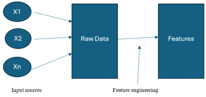
Figure 1. Feature Engineering Illustration.

2.3. Model Development

There are different types of machine learning algorithm used in prediction. The most common and popular among them are Linear Regression, SVM, Random Forest, Xgboost, and Gradient Boosting

[36]

. In this study, Google Colab was used to build the regression models which are Random Forest and Gradient Boosting to forecast daily oil production rates using historical operational and production data.

In this study, Google Colab was used to build the regression models to forecast daily oil production rates using historical operational and production data. The dataset was split into 75:25 for training and testing. The regression models were developed using the Python programming language, utilizing the cleaned dataset obtained from the data preprocessing stage phase was loaded into Python using Google Colab. Python based scikit-learn library’s RandomForestRegressor and GradientBoostingRegressor were used to develop the RFR and GBR algorithm. After which relevant predictor variables were selected based on physical relevance and correlation analysis.

Random Forest models were developed by tuning the depth of the trees, the number of trees, and the splitting rules to reduce prediction variability while avoiding overfitting. Increasing the number of trees helps prevent overfitting and improves the accuracy of the model’s predictions

[37]

. Table 1 shows some hyperparameters for Random Forest and Gradient Boosting algorithm and their default value. In contrast, Gradient Boosting models were built using shallow trees, carefully selected learning rates, and subsampling to gradually improve predictions by correcting errors from previous iterations. The final models were trained on historical production data and evaluated using several performance measures and residual analyses to confirm their reliability and ability to generalize for short-term oil production forecasting.

Table 1. Some Hyperparameters of Random Forest and Gradient Boosting algorithm and their default values.

Hyperparameter	Random Forest	Gradient Boosting
n_estimators	100	100
max_depth	None	3
min_samples_split	2	2
min_samples_leaf	1	1
learning_rate	NA	0.1
subsample	NA	1.0

Instead of relying on the default hyperparameters provided by the scikit-learn library, hyperparameter optimization was performed to achieve the primary objectives of the study.

2.4. Hyperparameter Optimization

The hyperparameter optimization plays a crucial role in enhancing the predictive accuracy of machine learning and deep learning models by selecting the optimal parameters for a given model. It is a widely adopted practice for developing robust and reliable ML models

[38]

. Several hyperparameter tuning techniques exist, including Grid Search, Bayesian Optimization, and Random Search. This process involves fine-tuning algorithm parameters to achieve the best-performing models

[39]

In recent years, several algorithms have been developed to optimize hyperparameter values, including Random Search, Grid Search, model-based approaches such as Random Forest, and sequential model-based optimization

[40]

. In this study, rather than using the default hyperparameters assigned by scikit-lean library, to achieve the primary objectives of the study, hyperparameter optimization was implemented. Hyperparameter optimization is a commonly used practice to build robust ML models

[41]

. Specifically, the hyperparameters of the Random Forest Regressor (RFR) were tuned using the Random Search method, implemented via the RandomizedSearchCV function in the scikit-learn library. Random Search Optimisation was considered with 50 combinations (n_iter) in the hyperparameter space using negative MSE

[42]

Download: Download full-size image

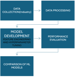
Figure 2. Methodology Workflow.

2.4.1. Random Forest

Random Forest is a supervised machine learning algorithm widely used due to its simplicity and versatility in both regression and classification tasks. First proposed by Leo Breiman at the University of California in 2001, the algorithm operates by training multiple decision tree models on input data, aggregating their predictions, and employing a voting or averaging process to produce the final output. This ensemble approach, also known as Random Decision Forests, improves prediction accuracy by combining the outputs of multiple trees

[43]

\hat{y} = \frac{1}{k} \sum_{k = 1}^{K} h_{k} (x)

(2)

where

h_{k} (x)

represents the prediction from the

k

-th decision tree and

K

is the total number of trees in the forest.

2.4.2. Gradient Boosting

Gradient Boosting Regression (GBR) is a supervised learning technique that iteratively improves model performance by learning from the errors of previous models. Introduced by Jerome H. Friedman in 2001

[44]

, it is a boosting method that combines multiple weak learners, typically decision trees, in a sequential manner. Each subsequent learner is trained on a modified version of the dataset, where adjustments are made based on the prediction errors of the preceding learner, allowing the ensemble to progressively enhance overall predictive accurate.

\hat{y} = \sum_{k = 1}^{K} {η h}_{k} (x)

(3)

where:

h_{k} (x)

is the prediction from the

k

-th weak learner,

K

is the total number of trees,

η

is the learning rate, which controls the contribution of each tree to the final prediction.

2.5. Performance Evaluation

Model evaluation extends beyond assessing accuracy, encompassing the overall reliability of predictions. Both accuracy and reliability are essential for effective forecasting. To evaluate the predictive performance of machine learning models, several studies have employed metrics such as Mean Squared Error (MSE), Root Mean Squared Error (RMSE), Mean Absolute Error (MAE), Mean Absolute Percentage Error (MAPE), and R-squared (R²)

[45]

. The performance of the models was assessed using the unseen test data by using the following performance metrics to ensure a robust and objective assessment.

2.5.1. Mean Absolute Error (MAE)

This metric will provide the average of all absolute errors between predicted and actual values. It will help in understanding the typical magnitude of the model’s errors in practical units such as barrels (bbl) or thousand standard cubic feet (mscf). An ideal value is 0, whereas the worst-case scenario corresponds to positive infinity

[46]

MAE = \frac{1}{N} \sum_{i = 1}^{N} |y_{reali} - y_{predi}|

(4)

2.5.2. Root Mean Squared Error (RMSE)

The Root Mean Squared Error (RMSE) measures the differences between actual and predicted values, aggregating these differences to evaluate a model’s forecasting performance. A smaller RMSE indicates better predictive accuracy. RMSE is particularly sensitive to outliers, as it assigns greater weight to errors with larger magnitudes compared to those with smaller deviations

[47]

. The root mean square error tells you, on average how far the model’s predictions are from the actual values, with errors squared to penalize large deviations.

RMSE = \sqrt{\frac{1}{N} {\sum_{i = 1}^{N} (y_{rea l_{i}} - y_{pre d_{i}})}^{2}}

(5)

2.5.3. Coefficient of Determination (R²)

R-squared (R²) is a straightforward metric for evaluating model performance, ranging from 0 to 1, with a value of 1 indicating a perfect fit between predicted and actual values. An R² score closer to 1 will suggest that the model captures the underlying trends and patterns effectively

[48]

R^{2} = 1 - \frac{\sum_{i = 1}^{N} {(y_{rea l_{i}} - y_{pre d_{i}})}^{2}}{\sum_{i = 1}^{N} {(y_{rea l_{i}} - \overset{̅}{y})}^{2}}

(6)

3. Results and Discussion

3.1. Correlation Analysis Results

In this study, Pearson correlation analysis was used to calculate the relationship between each variable in the dataset. The analysis was performed between the target variable, oil_rate and predictor variables: liquid_rate, gas_rate, water_rate, water_cut, tubing_head_pressure, choke_size, gas_oil_ratio, and days_on_production. Liquid_rate showed a strong positive correlation with oil_rate across well 1 and 2 as shown in Figures 3 and 4 respectively, reflecting the coupled flow of oil and liquid production. Tubing_head_pressure and days_on_production showed negative correlations in well 2, 3 and 4 as shown in Figures 4, 5 and 6 respectively. Multicollinearity was detected in several wells; Liquid_rate and water_rate in Wells 3 and 4 as shown in Figures 5 and 6 respectively. Gas_rate and gas_oil_ratio (GOR) in Wells 2, 3 and 4 as shown in Figures 4, 5 and 6 respectively. The relevance of features serves as a crucial basis for variable selection in Random Forest models. Removing redundant or low-importance features that exhibit weak correlation with the target variable can enhance the efficiency and performance of the model

[49]

The Pearson’s Correlation Matrix for each well is shown in Figures 3 to 6 below:

Download: Download full-size image

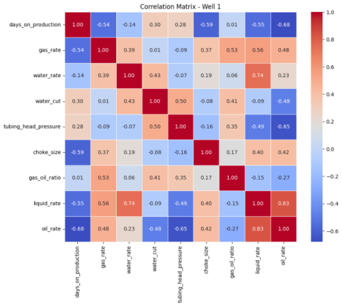
Figure 3. Pearson’s Correlation Matrix Heat Map for Well 1.

Download: Download full-size image

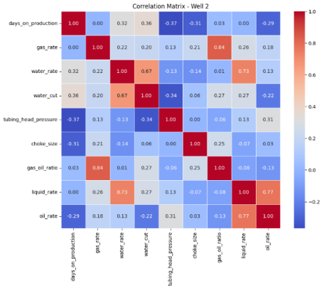
Figure 4. Pearson’s Correlation Matrix Heat Map for Well 2.

Download: Download full-size image

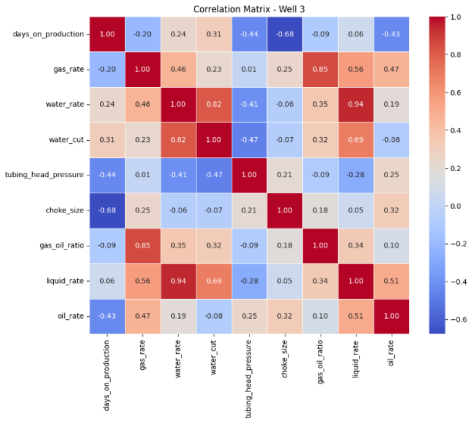
Figure 5. Pearson’s Correlation Matrix Heat Map for Well 3.

Download: Download full-size image

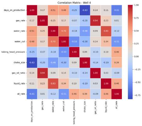
Figure 6. Pearson’s Correlation Matrix Heat Map for Well 4.

3.2. Hyperparameter Optimization

In this study, RandomisedSearch with 5-fold Cross Validation was used to select the best parameters. Grid Search is commonly employed for linear regression models, while Random Search is typically preferred for tuning Random Forest algorithms. For models such as Support Vector Regression (SVR), XGBoost, and Gradient Boosting, Bayesian optimization is generally recommended. RandomizedSearchCV was used to perform hyperparameter tuning for both the Random Forest and Gradient Boosting models, offering a more computationally efficient alternative to Grid Search

[50]

. The procedure evaluated 50 randomly selected hyperparameter combinations, including the number of estimators, maximum tree depth, minimum samples required for node splits and leaf nodes, and the use of bootstrap sampling. Hyperparameter tuning was performed using 5-fold cross-validation with negative Mean Squared Error (MSE) as the scoring metric, the optimal hyperparameters are shown in Table 2.

Wells with more irregular production patterns, such as Well 3, produced better results when larger minimum leaf sizes were applied, as this helped the model focus on general trends rather than random fluctuations. From the results, Well 2, which had a steadier production pattern, did better with deeper trees and more estimators. For the Gradient Boosting model, shallow trees with lower learning rates gave the best results, helping the model improve predictions gradually. Using subsampling also reduced overfitting, especially in wells with noisy production, such as Well 4. The model’s hyperparameters can be tailored to the dataset to enhance predictive accuracy and overall performance

[51]

. The hyperparameters of each well and model is shown in Table 2 below.

Table 2. Hyperparameters for Random Forest and Gradient Boosting.

Well	Model	Hyperparameters
1	RF	n_estimators=300, max_depth=15, min_samples_split=2, min_samples_leaf=1
	GB	n_estimators=300, max_depth=3, learning_rate=0.05, subsample=0.8
2	RF	n_estimators=100, max_depth=None, min_samples_split=2, min_samples_leaf=1
	GB	n_estimators=100, max_depth=5, learning_rate=0.01, subsample=0.9
3	RF	n_estimators=200, max_depth=15, min_samples_split=5, min_samples_leaf=4
	GB	n_estimators=100, max_depth=3, learning_rate=0.1, subsample=0.8
4	RF	n_estimators=200, max_depth=15, min_samples_split=2, min_samples_leaf=2
	GB	n_estimators=300, max_depth=3, learning_rate=0.1, subsample=0.9

3.3. Model Performance Evaluation

The performance metrics evaluation summarized in Table 3, which are Coefficient of Determination (

R^{2}

), Root Mean Squared Error (RMSE) and Mean Absolute Error (MAE).

3.3.1. Random Forest vs Gradient Boosting

Model performance metrics for the tuned and engineered models are summarized in Table 3 below:

Table 3. Model Performance Evaluation Results.

Well	Model	$R^{2}$	RMSE	MAE
Well 1	Random Forest	0.8508	25.7662	14.59871
Well 1	Gradient Boosting	0.9164	19.281	11.5872
Well 2	Random Forest	0.8275	59.2901	45.84983
Well 2	Gradient Boosting	0.8767	48.3085	39.9508
Well 3	Random Forest	0.7803	101.4342	56.1928
Well 3	Gradient Boosting	0.8956	69.9055	33.4839
Well 4	Random Forest	0.9756	26.5602	14.3022
Well 4	Gradient Boosting	0.9887	18.0494	7.9243

With higher R² and lower RMSE/MAE in all wells (Well 1, 2, 3, and 4) as shown in Table 3, Gradient Boosting generally did better than Random Forest. In line with its more stable production profile, well 4 had the highest predicted accuracy (

R^{2}

= 0.9887). An R² value approaching 1 indicates that the model demonstrates strong predictive performance. From the results, Well 3 has a significantly lower

R^{2}

(RF: 0.78, GB: 0.89), probably as a result of greater unpredictability and irregular periods of zero production. Also, the Figures 7 to 10 shows the actual oil rate vs. forecasted oil rate of the tuned and engineered features of the Random Forest and Gradient Boosting machine learning models.

Download: Download full-size image

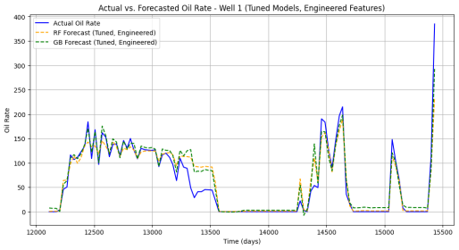
Figure 7. Actual vs. Forecasted (RF and GB) Oil Rate for Well 1.

Download: Download full-size image

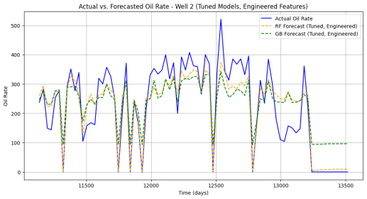
Figure 8. Actual vs. Forecasted (RF and GB) Oil Rate for Well 2.

Download: Download full-size image

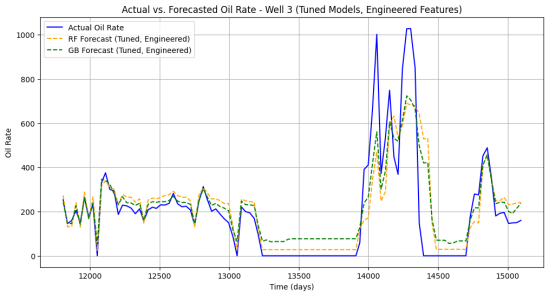
Figure 9. Actual vs. Forecasted (RF and GB) Oil Rate for Well 3.

Download: Download full-size image

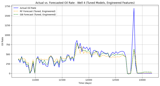
Figure 10. Actual vs. Forecasted (RF and GB) Oil Rate Well 4.

3.3.2. Analysis of Residuals to Investigate Autocorrelation and Model Assumptions

Residual analysis was performed for Random Forest and Gradient Boosting model. Some wells had moderate to high lag 1 autocorrelation (Well 1: 0.53 for RF, 0.47 for GB; Well 4: 0.75 for RF). Autocorrelation decreased with longer lags (7, 30 days) indicating that while the models may not adequately account for longer-term temporal patterns, they were able to capture the majority of short-term relationships.

According to its sequential residual-correcting technique, Gradient Boosting often decreased residual autocorrelation more successfully than Random Forest. Gradient Boosting generally reduced residual autocorrelation more effectively than Random Forest, consistent with its sequential residual-correcting mechanism. The Autocorrelation Function (ACF) quantifies the linear dependence between observations in a time series separated by a lag k. ACF and Partial Autocorrelation Function (PACF) plots are commonly used to assess the stationarity of a time series. If the ACF decreases rapidly after the first lag, the series is considered stationary. Conversely, if the ACF decays slowly, the series is non-stationary, and a differencing operation is required to achieve stationarity

[52]

. The autocorrelation of random forest and gradient boosting for all the wells are shown in Figures 11 to 14.

Download: Download full-size image

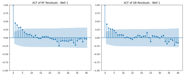
Figure 11. Autocorrelation function (ACF) of Residuals – Well 1.

Download: Download full-size image

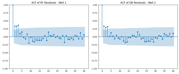
Figure 12. Autocorrelation function (ACF) of Residuals – Well 2.

Download: Download full-size image

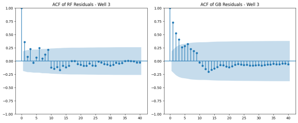
Figure 13. Autocorrelation function (ACF) of Residuals – Well 3.

Download: Download full-size image

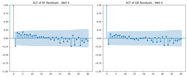
Figure 14. Autocorrelation function (ACF) of Residuals – Well 4.

4. Conclusion

In conclusion, this study shows the effectiveness and significance of the machine learning models developed for production forecasting in Niger Delta Oil Field through the following key findings:

1) The newly developed machine learning algorithms, particularly the Gradient Boosting model for well 4 was able to achieve the highest

R^{2}

value of 0.9887 and the lowest RMSE value of 18.0494 and lowest MSE value of 7.9243, which indicates that the model can provide accurate and robust oil rate forecasts for Niger Delta well, even in cases where the production profiles exhibit non-linearity, operational changes or noise.

2) Gradient Boosting model consistently outperformed Random Forest across all wells, showing lower error metrics across all the wells. This shows its suitability for capturing complex non-linear reservoir and operational conditions.

3) Wells with significant unstable production behaviour that is well 2 and 3 showed relatively lower performance metrics. It indicates that machine learning models struggle when operational changes or intermittent flow patterns exist in the dataset.

Although, the machine learning models performed well, the residuals still showed some correlation, which shows that certain reservoir behaviours were not fully captured. This suggests that future studies could benefit from using models that better account for time-dependent patterns.

Abbreviations

ANN	Artificial Neural Network
ARIMA	Autoregressive Integrated Moving Average
CV	Cross-Validation
DCA	Decline Curve Analysis
GB	Gradient Boosting
GOR	Gas–Oil Ratio
KNN	k-Nearest Neighbors
Lag-n	Time Lag of n Days
LSTM	Long Short-Term Memory
MAE	Mean Absolute Error
MSE	Mean Squared Error
ML	Machine Learning
RF	Random Forest
RMSE	Root Mean Squared Error
R²	Coefficient of Determination
SVR	Support Vector Regression
SVM	Support Vector Machine

Acknowledgments

The authors express their sincere appreciation to the Department of Petroleum Engineering of Abubakar Tafawa Balewa University Bauchi, for their unwavering support and provision of essential resources throughout this research work.

Author Contributions

Haliru Kawule Haliru: Conceptualization, Methodology, Software, Writing – original draft

Shamsuddeen Abubakar Ashurah: Investigation, Supervision, Visualization

Ibrahim Ayuba: Resources, Software, Validation

Data Availability Statement

The data is available from the corresponding author upon reasonable request.

Conflicts of Interest

The authors declare no conflicts of interest

References

[1]	Doan, T., & Van Vo, M. (2021). Using machine learning techniques for enhancing production forecast in the North Malay Basin. Proceedings of the International Field Exploration and Development Conference 2020 (pp. 114–121). Springer. https://doi.org/10.1007/978-981-16-0761-5_11
[2]	AlRassas, A. M., et al. (2021). Optimized ANFIS model using Aquila Optimizer for oil production forecasting. Processes, 9(7), 1194. https://doi.org/10.3390/pr9071194
[3]	Makhotin, I., Koroteev, D., & Burnaev, E. (2019). Gradient Boosting to Boost the Efficiency of Hydraulic Fracturing. Journal of Petroleum Exploration and Production Technology. https://link.springer.com/article/10.1007/s13202-019-0636-7
[4]	Ibrahim, N. M., et al. (2022). Well performance classification and prediction: Deep learning and machine learning long-term regression experiments on oil, gas, and water production. Sensors, 22(14), 5326. https://doi.org/10.3390/s22145326
[5]	Negash, B. M., & Yaw, A. D. (2020). Artificial neural network-based production forecasting for a hydrocarbon reservoir under water injection. Petroleum Exploration and Development, 47(2), 383–392. https://doi.org/10.1016/S1876-3804(20)60055-6
[6]	Arps, J. J. (1945). Analysis of Decline Curves. Transactions of the AIME, 160(1), 228–247.
[7]	Al-Fakih, A., Ibrahim, A. F., Elkatatny, S., & Abdulraheem, A. (2023). Estimating electrical resistivity from logging data for oil wells using machine learning. Journal of Petroleum Exploration and Production Technology, 13(6), 1453–1461. https://doi.org/10.1007/s13202-023-01617-2
[8]	Omotosho, T. J. (2024). Oil Production Prediction Using Time Series Forecasting and Machine Learning Techniques. Society of Petroleum Engineers - SPE Nigeria Annual International Conference and Exhibition, NAIC 2024. https://doi.org/10.2118/221728-MS
[9]	Tariq, Z., Aljawad, M. S., Hasan, A., Murtaza, M., Mohammed, E., El-Husseiny, A., Alarifi, S. A., Mahmoud, M., & Abdulraheem, A. (2021). A systematic review of data science and machine learning applications to the oil and gas industry. Journal of Petroleum Exploration and Production Technology 2021 11: 12, 11(12), 4339–4374. https://doi.org/10.1007/S13202-021-01302-2
[10]	Nekekpemi, Prosper; Totaro, Michael; Olayiwola, Olatunji; Esenenjor, Pascal 2024 Development of Machine Learning Models for Predicting Bubble-Point Pressure of Crude Oils https://doi.org/10.4043/35276-MS
[11]	Tadjer, A., Hong, A., & Bratvold, R. B. (2021). Machine learning based decline curve analysis for short-term oil production forecast. Energy Exploration and Exploitation, 39(5), 1747–1769. https://doi.org/10.1177/01445987211011784
[12]	Fan, D., Sun, H., Yao, J., Zhang, K., Yan, X., Sun, Z., 2021. Well production forecasting based on ARIMA-LSTM model considering manual operations. Energy 220, 119708. https://doi.org/10.1016/j.energy.2020.119708
[13]	Tan, C., et al. (2021). Fracturing productivity prediction model and optimization of the operation parameters of shale gas wells based on machine learning. Lithosphere, 2021(Special 4), 2884679. https://doi.org/10.2113/2021/2884679
[14]	Wang, X.-Y., Ma, Y.-J., Fei, E.-Z., & Gao, Y.-F. (2023). Daily production prediction of oil wells based on machine learning. In Proceedings of the International Conference on Automation Control, Algorithm, and Intelligent Bionics (ACAIB 2023) (Vol. 12759, pp. 516–520). SPIE. https://doi.org/10.1117/12.2686768
[15]	Ojedapo, B., Ikiensikimama, S. S., & Wachikwu-Elechi, V. U. (2022). Petroleum Production Forecasting Using Machine Learning Algorithms. Society of Petroleum Engineers - SPE Nigeria Annual International Conference and Exhibition, NAIC 2022. https://doi.org/10.2118/212018-MS
[16]	Jayeola, I., Alabi, M., & Ibrahim, A. (2022). Machine Learning Prediction Versus Decline Curve Prediction: A Niger Delta Case Study. SPE Nigeria Annual International Conference and Exhibition, OnePetro. https://onepetro.org/SPENAIC/proceedings-abstract/22NAIC/2-22NAIC/D021S009R002/495009
[17]	Song, X., et al. (2024). A comprehensive review of data-driven approache Artificial Intelligence Review.
[18]	Adewale, M. D., Adey (Placeholder 1) anju, I. A., Oju, J., Ubadike, O. C., Muhammed, U. I., & Omisakin, S. T. (2025). Ensemble machine learning methods to predict oil production. In Innovations and Interdisciplinary Solutions for Underserved Areas (INTERSOL). Springer. https://doi.org/10.1007/9783031864933_27eudl.eu
[19]	Shuqin Wen, Bing Wei, Junyu You, Yujiao He, Jun Xin, Mikhail A. Varfolomeev, Forecasting oil production in unconventional reservoirs using long short term memory network coupled support vector regression method: A case study, Petroleum, Volume 9, Issue 4, 2023, Pages 647-657, https://doi.org/10.1016/j.petlm.2023.05.004
[20]	Lee K, Lim J, Yoon D, et al. (2019) Prediction of shale-gas production at duvernay formation using deep-learning algorithm. SPE Journal 24(6): 2423–2437.
[21]	Ahmed Alsaihati, Mahmoud Abughaban, Salaheldin Elkatatny, and Dhafer Al Shehri Application of Machine Learning Methods in Modeling the Loss of Circulation Rate while Drilling Operation ACS Omega 2022, 7, 20696−20709.
[22]	Lee, J.; Wang, W.; Harrou, F.; Sun, Y. Reliable solar irradiance prediction using ensemble learning-based models: A comparative study. Energy Convers. Manag. 2020, 208, 112582.
[23]	Ayuba, I., Akanji, L. T., & Gomes, J. (2025). Numerical quantification of gas adsorption in unconventional shale rocks. Fuel, 396, 135246. https://doi.org/10.1016/j.fuel.2025.135246
[24]	Ayuba, I., Akanji, L. T., Gomes, J. L., & Falade, G. K. (2021). Investigation of drift phenomena at the pore scale during flow and transport in porous media. Mathematics, 9(19), 2509. https://doi.org/10.3390/math9192509
[25]	Salisu, A. M., Ayuba, I., Abdulrasheed, A., & Usman, A. (2025). Predicting liquid loading in gas condensate wells using machine learning to enhance production efficiency. Petroleum Science and Engineering, 9(2), 55–66 https://doi.org/10.11648/j.pse.20250902.12
[26]	Maharana K, Mondal S, Nemade B. A review: Data pre-processing and data augmentation techniques. Global Transitions Proceedings. 2022 Jun 1; 3(1): 91-9.
[27]	Suherman IC, Sarno R. Implementation of random forest regression for COCOMO II effort estimation. In 2020 international seminar on application for technology of information and communication (iSemantic) 2020 Sep 19 (pp. 476-481). IEEE.
[28]	Yilmazer S, Kocaman S. A mass appraisal assessment study using machine learning based on multiple regression and random forest. Land use policy. 2020 Dec 1; 99: 104889.
[29]	A. Jain, H. Patel, L. Nagalapatti, N. Gupta, S. Mehta, S. Guttula, S. Mujumdar, S. Afzal, R. Sharma Mittal and V. Munigala Overview and importance of data quality for machine learning tasks. InProceedings of the 26th ACM SIGKDD international conference on knowledge discovery & data mining 2020 Aug 23 (pp. 3561–3562).
[30]	Garcia-Carretero R, Holgado-Cuadrado R, Barquero-Pérez Ó. Assessment of classification models and relevant features on nonalcoholic steatohepatitis using random forest. Entropy. 2021 Jun 17; 23(6): 763.
[31]	Adeniyi EA, Gbadamosi B, Awotunde JB, Misra S, Sharma MM, Oluranti J (2022) Crude Oil Price Prediction Using Particle Swarm Optimization and Classi?cation Algorithms. 418 LNNS, 1384–1394. Scopus. https://doi.org/10.1007/978-3-030-96308-8_128
[32]	Moroff, N. U., Kurt, E., & Kamphues, J. (2021). Machine learning and statistics: A study for assessing innovative demand forecasting models. Procedia Computer Science, 180, 40–49. https://doi.org/10.1016/j.procs.2021.01.127
[33]	Schuetter J., Mishra S., Zhang M. and Lafollette R. (2015). Data Analytics for Production Optimization in Unconven- tional Reservoirs presented at Unconventional Resources Technology Conference, San Antonio, Texas, USA 2015. https://doi.org/10.15530/URTEC-2015-2167005
[34]	Shumway, R. and D. Stoffer. “Time Series Analysis and Its Applications: With R Examples.” ser. Springer Texts in Statistics. Springer New York, 2010. Available: https://books.google.com/books?id=dbS5IQ8P5gYC
[35]	Niu, W.; Lu, J.; Sun, Y. A Production Prediction Method for Shale Gas Wells Based on Multiple Regression. Energies 2021, 14, 1461.
[36]	G. S. Ohannesian and E. J. Harfash, "Epileptic Seizures Detection from EEG Recordings Based on a Hybrid system of Gaussian Mixture Model and Random Forest Classifier," Informatica, vol. 46, no. 6, 2022, https://doi.org/10.31449/inf.v46i6.4203
[37]	Friedman, J. Greedy function approximation: A gradient boosting machine. Ann. Stat. 2001, 29, 1189–1232.
[38]	Mo, H., Sun, H., Liu, J., & Wei, S. (2019). Developing window behavior models for residential buildings using XGBoost algorithm. Energy and Buildings, 205, 109564. https://doi.org/10.1016/j.enbuild.2019.109564
[39]	Alqahtani MG, Abdelhafez HA (2023) STOCK MARKET PREDICITION USING STATISTICAL & DEEP LEARNING TECHNIQUES. J Theoretical Appl Inform Technology 101(23): 7808–7825 Scopus.
[40]	Chicco, D., Warrens, M. J., & Jurman, G. (2021). The coefficient of determination R-squared is more informative than SMAPE, MAE, MAPE, MSE and RMSE in regression analysis evaluation. PeerJ Computer Science, 7, e623. https://doi.org/10.7717/peerj-cs.623
[41]	Dennis A. Huber, Jacob N. Persson, Forecasting Volatility: Evidence From The Swiss Stock Market. Master thesis at Lund university School of Economics and Managements 2010.
[42]	Eva Elling and Hannes Fornander, A Study of Recommender Techniques Within the Field of Collaborative Filtering. Thesis at KTH, School of Electrical Engineering, 2017.
[43]	Abbaszadeh M, Soltani-Mohammadi S, Ahmed AN. Optimization of support vector machine parameters in modeling of Iju deposit mineralization and alteration zones using particle swarm optimization algorithm and grid search method. Computers & Geosciences. 2022 Aug 1; 165: 105140.
[44]	Abbas MA, Al-Mudhafar WJ, Wood DA. Improving permeability prediction in carbonate reservoirs through gradient boosting hyperparameter tuning. Earth Science Informatics. 2023 Dec; 16(4): 3417-32.
[45]	Sandunil K, Bennour Z, Ben Mahmud H, Giwelli A. Effects of Tuning Hyperparameters in Random Forest Regression on Reservoir's Porosity Prediction. Case Study: Volve Oil Field, North Sea. InARMA US Rock Mechanics/Geomechanics Symposium 2023 Jun 25 (pp. ARMA-2023). ARMA.
[46]	Tao, Y. and Du, J. (2019) Temperature prediction using long short term memory network based on Random Forest [J]. Computer Engineering and Design, 40(03), 737-743.
[47]	Shen, P., Jin, Q., Zhou, Y., Xu, R. and Huang, H. (2022) Spatial-temporal pattern and driving factors of surface ozone concentrations in Zhejiang Province [J]. Research of Environmental Sciences, 35(09), 2136-2146.
[48]	Rimal Y, Sharma N, Alsadoon A (2024) The accuracy of machine learning models relies on hyperparameter tuning: student result classification using random forest, randomized search, grid search, bayesian, genetic, and optuna algorithms. Multimedia Tools Appl 83(30): 74349–74364.
[49]	Liu, D.; Sun, K. Random forest solar power forecast based on classification optimization. Energy 2019, 187, 115940.1–115940.11.
[50]	Tianrui Cai Stock Forecasting Based on Random Forest and ARIMA Models Proceedings of CONF-MPCS 2025 Symposium: Mastering Optimization: Strategies for Maximum Efficiency https://doi.org/10.54254/2753-8818/101/2025.CH22310
[51]	Hyndman, R. J., & Athanasopoulos, G. (2018) Forecasting: principles and practice, 2nd edition, OTexts: Melbourne, Australia. OTexts.com/fpp2
[52]	Haseen. Forecasting Crude Oil Prices: Insights from Machine Learning Approaches, 16 December 2025, PREPRINT (Version 1) available at Research Square https://doi.org/10.21203/rs.3.rs-8354755/v1

Cite This Article

Plain Text BibTeX RIS

APA Style

Haliru, H. K., Ashurah, S. A., Ayuba, I. (2026). Application of Machine Learning for Production Forcasting in Niger Delta Oil Field (Ozoro Field). Petroleum Science and Engineering, 10(1), 1-16. https://doi.org/10.11648/j.pse.20261001.11

Copy | Download

ACS Style

Haliru, H. K.; Ashurah, S. A.; Ayuba, I. Application of Machine Learning for Production Forcasting in Niger Delta Oil Field (Ozoro Field). Pet. Sci. Eng. 2026, 10(1), 1-16. doi: 10.11648/j.pse.20261001.11

Copy | Download

AMA Style

Haliru HK, Ashurah SA, Ayuba I. Application of Machine Learning for Production Forcasting in Niger Delta Oil Field (Ozoro Field). Pet Sci Eng. 2026;10(1):1-16. doi: 10.11648/j.pse.20261001.11

Copy | Download

@article{10.11648/j.pse.20261001.11,
  author = {Haliru Kawule Haliru and Shamsuddeen Abubakar Ashurah and Ibrahim Ayuba},
  title = {Application of Machine Learning for Production Forcasting in Niger Delta Oil Field (Ozoro Field)},
  journal = {Petroleum Science and Engineering},
  volume = {10},
  number = {1},
  pages = {1-16},
  doi = {10.11648/j.pse.20261001.11},
  url = {https://doi.org/10.11648/j.pse.20261001.11},
  eprint = {https://article.sciencepublishinggroup.com/pdf/10.11648.j.pse.20261001.11},
  abstract = {Daily oil production forecasts are a key part of how reservoirs are managed and how production plans are made in the upstream oil and gas industry. In practice, however, getting accurate daily forecasts is not always easy. This is very common in the Niger Delta region where wells are usually affected by shutdowns, flow interruptions and changing operational conditions. Because of these reasons, oil production data from these wells are usually irregular and traditional forecasting methods usually struggle to capture these changes. This study looks at whether machine learning models can do a better job of predicting daily oil production rates. Historical oil production data from four wells in a Niger Delta oilfield was used for the study. Two ensemble models which are random forest and gradient boosting were selected and tested. Before building the models, the data was checked carefully and cleaned. Some new variables were also created to help the models understand how production changes over time. Hyperparameter optimization was performed using RandomisedSearchCV with 5-fold cross-validation to choose the best model settings and to avoid the risk of overfitting. Their performance was assessed using Coefficient of Determination (R²), Root Measure Squared Error (RMSE), and Mean Absolute Error (MAE). From the results, Gradient Boosting performed better in most cases. Its R² values were generally between 0.8767 and 0.9887, while the Random Forest model produced values in the range of about 0.7803 to 0.9756. The best predictions were obtained for wells that showed relatively stable production behaviour. For wells with frequent shutdowns and more unstable production, both models recorded higher errors with random forest having the highest error across all wells. This shows that prediction becomes more difficult when production conditions change often. Even though, the overall results suggest that ensemble machine learning models, particularly Gradient Boosting, can provide useful and reasonably accurate daily oil production forecasts for Niger Delta fields. These models can therefore support better planning and operational decision-making in Nigeria’s upstream oil and gas sector.},
 year = {2026}
}

Copy | Download

TY - JOUR
T1 - Application of Machine Learning for Production Forcasting in Niger Delta Oil Field (Ozoro Field)
AU - Haliru Kawule Haliru
AU - Shamsuddeen Abubakar Ashurah
AU - Ibrahim Ayuba
Y1 - 2026/02/24
PY - 2026
N1 - https://doi.org/10.11648/j.pse.20261001.11
DO - 10.11648/j.pse.20261001.11
T2 - Petroleum Science and Engineering
JF - Petroleum Science and Engineering
JO - Petroleum Science and Engineering
SP - 1
EP - 16
PB - Science Publishing Group
SN - 2640-4516
UR - https://doi.org/10.11648/j.pse.20261001.11
AB - Daily oil production forecasts are a key part of how reservoirs are managed and how production plans are made in the upstream oil and gas industry. In practice, however, getting accurate daily forecasts is not always easy. This is very common in the Niger Delta region where wells are usually affected by shutdowns, flow interruptions and changing operational conditions. Because of these reasons, oil production data from these wells are usually irregular and traditional forecasting methods usually struggle to capture these changes. This study looks at whether machine learning models can do a better job of predicting daily oil production rates. Historical oil production data from four wells in a Niger Delta oilfield was used for the study. Two ensemble models which are random forest and gradient boosting were selected and tested. Before building the models, the data was checked carefully and cleaned. Some new variables were also created to help the models understand how production changes over time. Hyperparameter optimization was performed using RandomisedSearchCV with 5-fold cross-validation to choose the best model settings and to avoid the risk of overfitting. Their performance was assessed using Coefficient of Determination (R²), Root Measure Squared Error (RMSE), and Mean Absolute Error (MAE). From the results, Gradient Boosting performed better in most cases. Its R² values were generally between 0.8767 and 0.9887, while the Random Forest model produced values in the range of about 0.7803 to 0.9756. The best predictions were obtained for wells that showed relatively stable production behaviour. For wells with frequent shutdowns and more unstable production, both models recorded higher errors with random forest having the highest error across all wells. This shows that prediction becomes more difficult when production conditions change often. Even though, the overall results suggest that ensemble machine learning models, particularly Gradient Boosting, can provide useful and reasonably accurate daily oil production forecasts for Niger Delta fields. These models can therefore support better planning and operational decision-making in Nigeria’s upstream oil and gas sector.
VL - 10
IS - 1
ER -

Copy | Download

Author Information

Haliru Kawule Haliru

Department of Petroleum Engineering, Abubakar Tafawa Balewa University, Bauchi, Nigeria

Contact Email

http://orcid.org/0009-0002-7604-1397
Shamsuddeen Abubakar Ashurah

Department of Petroleum Engineering, Abubakar Tafawa Balewa University, Bauchi, Nigeria

http://orcid.org/0009-0006-6103-9971
Ibrahim Ayuba

Department of Petroleum Engineering, Abubakar Tafawa Balewa University, Bauchi, Nigeria

http://orcid.org/0000-0001-6887-6808

Download PDF

Submit an Article

Plain Text BibTeX RIS

APA Style

Haliru, H. K., Ashurah, S. A., Ayuba, I. (2026). Application of Machine Learning for Production Forcasting in Niger Delta Oil Field (Ozoro Field). Petroleum Science and Engineering, 10(1), 1-16. https://doi.org/10.11648/j.pse.20261001.11

Copy | Download

ACS Style

Haliru, H. K.; Ashurah, S. A.; Ayuba, I. Application of Machine Learning for Production Forcasting in Niger Delta Oil Field (Ozoro Field). Pet. Sci. Eng. 2026, 10(1), 1-16. doi: 10.11648/j.pse.20261001.11

Copy | Download

AMA Style

Haliru HK, Ashurah SA, Ayuba I. Application of Machine Learning for Production Forcasting in Niger Delta Oil Field (Ozoro Field). Pet Sci Eng. 2026;10(1):1-16. doi: 10.11648/j.pse.20261001.11

Copy | Download

@article{10.11648/j.pse.20261001.11,
  author = {Haliru Kawule Haliru and Shamsuddeen Abubakar Ashurah and Ibrahim Ayuba},
  title = {Application of Machine Learning for Production Forcasting in Niger Delta Oil Field (Ozoro Field)},
  journal = {Petroleum Science and Engineering},
  volume = {10},
  number = {1},
  pages = {1-16},
  doi = {10.11648/j.pse.20261001.11},
  url = {https://doi.org/10.11648/j.pse.20261001.11},
  eprint = {https://article.sciencepublishinggroup.com/pdf/10.11648.j.pse.20261001.11},
  abstract = {Daily oil production forecasts are a key part of how reservoirs are managed and how production plans are made in the upstream oil and gas industry. In practice, however, getting accurate daily forecasts is not always easy. This is very common in the Niger Delta region where wells are usually affected by shutdowns, flow interruptions and changing operational conditions. Because of these reasons, oil production data from these wells are usually irregular and traditional forecasting methods usually struggle to capture these changes. This study looks at whether machine learning models can do a better job of predicting daily oil production rates. Historical oil production data from four wells in a Niger Delta oilfield was used for the study. Two ensemble models which are random forest and gradient boosting were selected and tested. Before building the models, the data was checked carefully and cleaned. Some new variables were also created to help the models understand how production changes over time. Hyperparameter optimization was performed using RandomisedSearchCV with 5-fold cross-validation to choose the best model settings and to avoid the risk of overfitting. Their performance was assessed using Coefficient of Determination (R²), Root Measure Squared Error (RMSE), and Mean Absolute Error (MAE). From the results, Gradient Boosting performed better in most cases. Its R² values were generally between 0.8767 and 0.9887, while the Random Forest model produced values in the range of about 0.7803 to 0.9756. The best predictions were obtained for wells that showed relatively stable production behaviour. For wells with frequent shutdowns and more unstable production, both models recorded higher errors with random forest having the highest error across all wells. This shows that prediction becomes more difficult when production conditions change often. Even though, the overall results suggest that ensemble machine learning models, particularly Gradient Boosting, can provide useful and reasonably accurate daily oil production forecasts for Niger Delta fields. These models can therefore support better planning and operational decision-making in Nigeria’s upstream oil and gas sector.},
 year = {2026}
}

Copy | Download