Mathematical Modelling of Light Propagation in Optical Fibers: From Maxwell’s Equations to Split-Step Simulation of Dispersive and Nonlinear Pulse Dynamics

Randriana Heritiana Nambinina Erica; Ando Nirina Andriamanalina

doi:doi:10.11648/j.sdmath.20260102.12

Methodology Article |

| Peer-Reviewed

Mathematical Modelling of Light Propagation in Optical Fibers: From Maxwell’s Equations to Split-Step Simulation of Dispersive and Nonlinear Pulse Dynamics

Randriana Heritiana Nambinina Erica^*

, Ando Nirina Andriamanalina

Published in Science Discovery Mathematics (Volume 1, Issue 2)

Received: 10 October 2026 Accepted: 20 October 2026 Published: 31 October 2026

Views: Downloads:

Download PDF

Share This Article

Twitter
Linked In
Facebook

Abstract

Optical fibers carry most of the world’s long-distance data traffic, and reliable mathematical models are essential for designing, optimizing and teaching the systems built on them. This work presents a self-contained mathematical model of light propagation in single-mode optical fibers and its numerical implementation in Python. Starting from Maxwell’s equations, we derive the guided-mode eigenvalue problem of the step-index fiber, the frequency dependence of attenuation and chromatic dispersion from the Sellmeier equation and empirical loss models, and the nonlinear Schrödinger equation (NLSE) governing the slowly varying pulse envelope under the combined effects of loss, dispersion and the Kerr nonlinearity. Closed-form results for Gaussian pulse broadening, self-phase modulation (SPM) and soliton propagation are used as analytical benchmarks and combined with a symmetric split-step Fourier method (SSFM) for the numerical solution. The numerical scheme is validated against these analytical solutions to a relative accuracy better than 10^-12 for linear propagation, reproduces the expected number of SPM spectral peaks, preserves fundamental and third-order solitons over two soliton periods, and demonstrates the expected second-order convergence with step size. A link-level simulation of a 2.5 Gb/s amplified system, including amplifier noise, a square-law receiver and the resulting Q-factor, shows an optimum launch power that decreases from approximately +11 dBm to +5 dBm as the number of 80 km spans increases from three to six, illustrating the trade-off between noise accumulation and nonlinear distortion. The results show how a compact, physics-based model, implemented in a few dozen lines of code, reproduces the main performance trade-offs of fiber-optic transmission and provides a validated basis for further studies including polarization effects, Raman scattering and multi-channel transmission.

Published in	Science Discovery Mathematics (Volume 1, Issue 2)
DOI	10.11648/j.sdmath.20260102.12
Page(s)	54-63
Creative Commons	This is an Open Access article, distributed under the terms of the Creative Commons Attribution 4.0 International License (http://creativecommons.org/licenses/by/4.0/), which permits unrestricted use, distribution and reproduction in any medium or format, provided the original work is properly cited.
Copyright	Copyright © The Author(s), 2026. Published by Science Publishing Group

Keywords

Optical Fiber, Nonlinear Schrödinger Equation, Chromatic Dispersion, Self-phase Modulation, Solitons, Split-step Fourier Method, Q-factor

1. Introduction

Optical fibers form the backbone of modern telecommunications and carry the overwhelming majority of intercontinental data traffic. The concept of guiding light in a dielectric waveguide for communication was proposed by Kao and Hockham

[1]

, and the fabrication of silica fibers with a loss below 20 dB/km by Kapron et al.

[2]

turned the idea into a practical technology. Today, attenuation in standard single-mode fiber (SMF) is close to 0.2 dB/km near 1550 nm. Combined with erbium-doped fiber amplifiers

[3]

and wavelength-division multiplexing, this low loss allows a single fiber to transmit tens of terabits per second. The achievable capacity is, however, ultimately bounded by amplifier noise and by the Kerr nonlinearity of silica

[4]

Designing and optimizing such systems requires reliable mathematical models. The modelling hierarchy is well established

[5, 6]

. At the most fundamental level, Maxwell’s equations determine the transverse mode profiles and propagation constants of the waveguide. For narrowband pulses, the field can be written as a slowly varying envelope multiplying a guided mode, and the evolution of this envelope is governed by a nonlinear partial differential equation, the nonlinear Schrödinger equation, which accounts for loss, chromatic dispersion and the Kerr effect. The NLSE has remarkable analytical properties: Hasegawa and Tappert showed that it supports stable solitary waves in the anomalous dispersion regime

[7]

, and Mollenauer et al. observed optical solitons experimentally

[8]

. For general input pulses, however, the NLSE must be solved numerically, most commonly with the split-step Fourier method

[9]

The purpose of this article is threefold. First, we give a compact and consistent derivation of the model, from the electromagnetic foundations to the numerical algorithm, with every equation written in a form that can be directly reused in simulation code. Second, we implement the model in Python and validate it against analytical benchmarks. Third, we use the validated tool to quantify the performance of a realistic amplified link, in terms of pulse broadening, spectral broadening, soliton stability, numerical accuracy and Q-factor. The paper is organized as follows: Section 2 describes the mathematical models and numerical methods, Section 3 presents the simulation results, Section 4 discusses their physical meaning and limitations, and Section 5 concludes.

2. Materials and Methods

2.1. Electromagnetic Foundations and Guided Modes

In a source-free, non-magnetic dielectric such as silica glass, Maxwell’s equations take the form

\nabla \times E = - \frac{\partial B}{\partial t}, \nabla \times H = \frac{\partial D}{\partial t}

(1)

where the constitutive relations are

D = ε_{0} E + P, B = μ_{0} H

(2)

and

P

is the induced polarization. Eliminating

B

and

H

and using

\nabla \cdot D = 0

yields the wave equation

[5]

\nabla^{2} E - \frac{1}{c^{2}} \frac{\partial^{2} E}{\partial t^{2}} = μ_{0} \frac{\partial^{2} P}{\partial t^{2}}

(3)

In the linear regime,

P

is related to

E

through the susceptibility

χ^{(1)} (ω)

, and in the frequency domain the wave equation reduces to the Helmholtz equation

\nabla^{2} \tilde{E} + n^{2} (ω) \frac{ω^{2}}{c^{2}} \tilde{E} = 0

(4)

with

n (ω) = \sqrt{1 + Re χ^{(1)} (ω)}

. For a step-index fiber with core radius

a

, core index

n_{1}

and cladding index

n_{2}

, the guiding properties depend on the normalized frequency

[10]

V = k_{0} a \sqrt{n_{1}^{2} - n_{2}^{2}} = \frac{2 πa}{λ} NA

(5)

where

k_{0} = 2 π / λ

and NA is the numerical aperture. The normalized propagation constant is defined as

b = \frac{β^{2} / k_{0}^{2} - n_{2}^{2}}{n_{1}^{2} - n_{2}^{2}} = \frac{w^{2}}{V^{2}}, u^{2} + w^{2} = V^{2}

(6)

where

β

is the propagation constant,

u = a \sqrt{k_{0}^{2} n_{1}^{2} - β^{2}}

and

w = a \sqrt{β^{2} - k_{0}^{2} n_{2}^{2}}

. In the weakly guiding approximation (

n_{1} - n_{2} ≪ n_{1}

) the modes are linearly polarized (LP

​_{lm}

) and satisfy the eigenvalue equation

[11]

u \frac{J_{l - 1} (u)}{J_{l} (u)} = - w \frac{K_{l - 1} (w)}{K_{l} (w)}

(7)

where

J_{l}

and

K_{l}

are the Bessel function of the first kind and the modified Bessel function of the second kind of order

l

. Only the fundamental LP

​_{01}

mode propagates when

V < 2.405

, the first zero of

J_{0}

; this is the single-mode condition used in all telecommunication fibers. Equation (7) was solved numerically with Brent’s root-finding algorithm applied to a regularized form of the characteristic function, which avoids the poles of the ratio of Bessel functions.

2.2. Attenuation and Chromatic Dispersion

Power decays exponentially as

P (z) = P_{0} e^{- αz}

along the fiber. Fiber manufacturers quote the loss in decibels per kilometer, related to the attenuation coefficient

α

(in km

​^{- 1}

) by

α_{dB} = - \frac{10}{L} \log_{10} \frac{P_{out}}{P_{in}} = 4.343 α

(8)

Because the mode propagation constant depends on frequency, different spectral components travel at different group velocities. Expanding

β (ω)

around the carrier frequency

ω_{0}

gives

[5]

β (ω) = β_{0} + β_{1} (ω - ω_{0}) + \frac{β_{2}}{2} {(ω - ω_{0})}^{2} + \frac{β_{3}}{6} {(ω - ω_{0})}^{3} + \dots, β_{m} = {\frac{d^{m} β}{d ω^{m}}|}_{ω = ω_{0}}

(9)

where

β_{1} = 1 / v_{g}

is the inverse group velocity and

β_{2}

is the group-velocity dispersion (GVD) parameter. The dispersion parameter commonly used in the telecommunication literature is

D = - \frac{2 πc}{λ^{2}} β_{2}

(10)

so that

D > 0

(anomalous dispersion,

β_{2} < 0

) holds in silica fibers above the zero-dispersion wavelength near 1.3 µm. The material contribution was computed from the three-term Sellmeier equation for fused silica

[12]

n^{2} (λ) = 1 + \sum_{j = 1}^{3} \frac{B_{j} λ^{2}}{λ^{2} - λ_{j}^{2}}, D_{M} = - \frac{λ}{c} \frac{d^{2} n}{d λ^{2}}

(11)

while the total dispersion of a standard G.652 fiber was described by the empirical form recommended by the ITU-T

[13]

D (λ) = \frac{S_{0}}{4} (λ - \frac{λ_{0}^{4}}{λ^{3}})

(12)

with

λ_{0} = 1312

nm and

S_{0} = 0.092

ps nm

​^{- 2}

​^{- 1}

. The spectral attenuation was represented by the sum of the main intrinsic and extrinsic contributions

[2, 14]

α_{dB} (λ) = \frac{C_{R}}{λ^{4}} + A_{IR} e^{- B_{IR} / λ} + α_{UV} + α_{OH} (λ)

(13)

where the four terms stand for Rayleigh scattering (

C_{R} = 0.75

dB µm

​^{4}

/km), infrared absorption (

A_{IR} = 7.81 \times 10^{11}

dB/km,

B_{IR} = 48.48

µm), a constant residual term and Gaussian hydroxyl-ion absorption peaks at 1.24 and 1.38 µm.

2.3. Nonlinear Pulse Propagation Equation

At high intensity, the refractive index of silica depends on the optical intensity

I

through the third-order susceptibility

χ^{(3)}

[15, 16]

n = n_{0} + n_{2} I, γ = \frac{2 π n_{2}}{λ A_{eff}}

(14)

where

n_{2} \approx 2.6 \times 10^{- 20}

​^{2}

/W is the nonlinear-index coefficient of silica,

A_{eff}

is the effective mode area and

γ

is the nonlinear parameter in W

​^{- 1}

​^{- 1}

. Writing the electric field as a slowly varying envelope

A (z, t)

times the fundamental mode and the carrier, and working in a frame moving at the group velocity (

T = t - β_{1} z

), one obtains the nonlinear Schrödinger equation

[5]

\frac{\partial A}{\partial z} + \frac{α}{2} A + \frac{i β_{2}}{2} \frac{\partial^{2} A}{\partial T^{2}} - \frac{β_{3}}{6} \frac{\partial^{3} A}{\partial T^{3}} = iγ {|A|}^{2} A

(15)

where

{|A|}^{2}

is the instantaneous optical power in watts. Two characteristic lengths measure the relative importance of dispersion and nonlinearity for a pulse of width

T_{0}

and peak power

P_{0}

L_{D} = \frac{T_{0}^{2}}{|β_{2}|}, L_{NL} = \frac{1}{γ P_{0}}, N^{2} = \frac{L_{D}}{L_{NL}} = \frac{γ P_{0} T_{0}^{2}}{|β_{2}|}

(16)

Introducing

ξ = z / L_{D}

τ = T / T_{0}

and

A = \sqrt{P_{0}} U

, the lossless NLSE takes the universal form

i \frac{\partial U}{\partial ξ} = \frac{sgn (β_{2})}{2} \frac{\partial^{2} U}{\partial τ^{2}} - N^{2} {|U|}^{2} U

(17)

which depends only on the soliton order

N

and on the sign of

β_{2}

. For

β_{2} < 0

the equation is integrable by the inverse scattering transform

[17]

2.4. Analytical Benchmark Solutions

Gaussian pulse in the linear regime. For an initially chirped Gaussian pulse

A (0, T) = \sqrt{P_{0}} \exp [- \frac{1 + iC}{2} \frac{T^{2}}{T_{0}^{2}}],

(18)

where

C

is the chirp parameter, the NLSE with

γ = α = β_{3} = 0

can be solved exactly. The pulse remains Gaussian and its width evolves as

[5]

\frac{T_{1}}{T_{0}} = \sqrt{{(1 + \frac{C β_{2} z}{T_{0}^{2}})}^{2} + {(\frac{β_{2} z}{T_{0}^{2}})}^{2}}

(19)

Initial narrowing occurs when

C β_{2} < 0

, with a minimum width

T_{0} / \sqrt{1 + C^{2}}

reached at

z = |C| L_{D} / (1 + C^{2})

Fundamental soliton. For

β_{2} < 0

and

N = 1

the NLSE (neglecting loss) has the exact solution

A (z, T) = \sqrt{P_{0}} sech ​ (\frac{T}{T_{0}}) \exp (\frac{iz}{2 L_{D}}), P_{0} = \frac{|β_{2}|}{γ T_{0}^{2}}

(20)

whose shape is invariant during propagation. Higher-order solitons (

N = 2, 3, \dots

) evolve periodically with the soliton period

z_{0} = π L_{D} / 2

[7]

Self-phase modulation. For

β_{2} = 0

the nonlinear term only modifies the phase of the pulse,

ϕ_{NL} (L, T) = γ L_{eff} {|A (0, T)|}^{2}, L_{eff} = \frac{1 - e^{- αL}}{α}

(21)

which produces a time-dependent frequency shift (chirp)

δω (T) = - \frac{\partial ϕ_{NL}}{\partial T}

(22)

and a broadened, oscillatory spectrum. For a smooth pulse the number

M

of spectral peaks is related to the maximum nonlinear phase by

[16]

ϕ_{\max} \approx (M - \frac{1}{2}) π

(23)

2.5. Split-step Fourier Method

For arbitrary inputs, Eq. (15) is solved numerically. It is written as

\partial A / \partial z = (\hat{D} + \hat{N}) A

with the linear and nonlinear operators

\hat{D} = - \frac{α}{2} - \frac{i β_{2}}{2} \frac{\partial^{2}}{\partial T^{2}} + \frac{β_{3}}{6} \frac{\partial^{3}}{\partial T^{3}}, \hat{N} = iγ {|A|}^{2}

(24)

The SSFM

[9]

advances the field over a small step

h

by applying the two operators alternately. In its symmetric form, equivalent to Strang splitting

[18]

A (z + h, T) \approx \exp (\frac{h}{2} \hat{D}) \exp (h \hat{N}) \exp (\frac{h}{2} \hat{D}) A (z, T)

(25)

The dispersion operator is applied in the frequency domain, where the time derivatives become algebraic factors and the fast Fourier transform (FFT) is used for efficiency:

\exp (\frac{h}{2} \hat{D}) B = F^{- 1} \{\exp [\frac{h}{2} (\frac{i β_{2}}{2} ω^{2} + \frac{i β_{3}}{6} ω^{3} - \frac{α}{2})] F {B}\}

(26)

The step size is selected so that the nonlinear phase accumulated per step remains small

[19]

Δ ϕ_{NL} = γ P_{peak} h \leq ϕ_{tol} \approx 0.05 rad

(27)

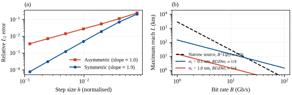
The symmetric scheme has a local error of order

h^{3}

and a global error of order

h^{2}

, whereas the asymmetric scheme (a single dispersion step followed by a single nonlinear step) is only first-order accurate. The numerical error was quantified as the relative

L_{2}

distance to a reference solution computed with a very small step

h_{ref}

ε (h) = \frac{{∥A_{h} - A_{ref}∥}_{2}}{{∥A_{ref}∥}_{2}} \propto h^{p}

(28)

where

p = 2

is expected for the symmetric and

p = 1

for the asymmetric scheme. A minimal Python implementation of the symmetric scheme is given in Listing 1.

import numpy as np def ssfm(A0, T, z, nsteps, beta2, gamma, alpha=0.0): """Symmetric SSFM. Units: T [ps], z [km], beta2 [ps^2/km], gamma [1/(W km)], alpha [1/km]; A0 in sqrt(W).""" w = 2*np.pi*np.fft.fftfreq(len(T), d=T[1]-T[0]) # rad/ps h = z/nsteps half = np.exp((1j*beta2/2*w**2 - alpha/2)*h/2) # exp(h/2 D) A = A0.astype(complex) for _ in range(nsteps): A = np.fft.ifft(half*np.fft.fft(A)) # half linear step A = A*np.exp(1j*gamma*np.abs(A)**2*h) # full nonlinear step A = np.fft.ifft(half*np.fft.fft(A)) # half linear step return A

Listing 1. Core of the symmetric split-step Fourier solver used in this work.

2.6. Link-level Performance Model

To assess system performance, a 2.5 Gb/s non-return-to-zero (NRZ) signal was propagated through

N_{s}

identical spans of 80 km of SMF, each followed by an erbium-doped fiber amplifier (EDFA) whose gain exactly compensates the span loss. Each amplifier adds amplified spontaneous emission (ASE) noise, modelled as circular complex Gaussian noise with power

P_{ASE} = n_{sp} (G - 1) hν Δν, NF \approx 2 n_{sp}

(29)

where

G

is the amplifier gain,

hν

the photon energy,

Δν

the simulation bandwidth and

n_{sp}

the spontaneous-emission factor (noise figure NF = 5 dB). At the receiver, the field passes through a Gaussian optical filter, a square-law photodetector and a Gaussian electrical filter with a bandwidth of

0.75 B

. The signal quality is evaluated at the center of each bit with the Q-factor, which is directly related to the bit-error ratio (BER),

Q = \frac{μ_{1} - μ_{0}}{σ_{1} + σ_{0}}, BER = \frac{1}{2} erfc ​ (\frac{Q}{\sqrt{2}})

(30)

where

μ_{1, 0}

and

σ_{1, 0}

are the mean and standard deviation of the received samples for logical ones and zeros. A value

Q = 15.6

dB corresponds to BER

\approx 10^{- 9}

. Finally, simple analytical reach limits were used for comparison: a transform-limited source is limited by

B^{2} L |β_{2}| ≲ 1 / 16

, while a source with rms spectral width

σ_{λ}

is limited by

[6]

BL |D| σ_{λ} ≲ \frac{1}{4}

(31)

2.7. Numerical Implementation and Parameters

All simulations were implemented in Python 3 using NumPy (FFT and array operations), SciPy (Bessel functions and root finding) and Matplotlib (figures). The parameters listed in Table 1 correspond to a standard G.652 fiber operated at 1550 nm. Pulse-propagation studies used a temporal grid of

2^{13}

points; the link simulation used 256 random bits with 32 samples per bit (also

2^{13}

points), a 1 km step, and four noise realizations averaged for each launch power. Polarization effects, Raman scattering and third-order dispersion were neglected in the simulations (

β_{3} = 0

Table 1. Fiber and simulation parameters (standard SMF at 1550 nm).

Parameter	Symbol	Value
Wavelength	$λ_{0}$	1550 nm
Dispersion parameter	$D$	17 ps nm $^{- 1}$ km $^{- 1}$
GVD coefficient	$β_{2}$	−21.68 ps $^{2}$ km $^{- 1}$
Nonlinear parameter	$γ$	1.3 W $^{- 1}$ km $^{- 1}$
Attenuation	$α_{dB}$	0.2 dB km $^{- 1}$
Gaussian pulse width	$T_{0}$	25 ps
Dispersion length	$L_{D}$	28.8 km
Span length / amplifier noise figure	$L_{s}$ / NF	80 km / 5 dB
Bit rate (NRZ)	$B$	2.5 Gb/s

3. Results

3.1. Guided modes, Attenuation and Dispersion

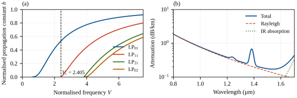
Figure 1(a) shows the normalized propagation constant

b

of the first LP modes as a function of

V

. The LP

​_{01}

mode has no cutoff, whereas LP

​_{11}

appears at

V = 2.405

; the next modes (LP

​_{21}

and LP

​_{02}

) appear at

V \approx 3.83

, in agreement with the zeros of the Bessel functions. Figure 1(b) presents the modelled spectral attenuation. The total loss reaches its minimum of 0.17 dB/km at 1.55 µm, where Rayleigh scattering and infrared absorption are balanced, and displays the characteristic OH

​^{-}

absorption peak at 1.38 µm.

Download: Download full-size image

Figure 1. (a) Normalized propagation constant

b

versus normalized frequency

V

for the first LP modes of a step-index fiber. (b) Modelled spectral attenuation of silica fiber and its main contributions.

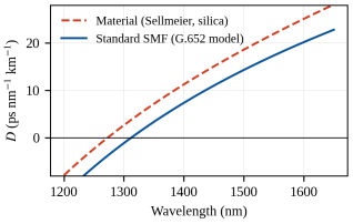
The dispersion curves are shown in Figure. 2. The material dispersion of silica computed from the Sellmeier equation is zero near 1.27 µm and equals 21.9 ps nm

​^{- 1}

​^{- 1}

at 1550 nm. Waveguide dispersion shifts the zero-dispersion wavelength of a standard fiber to about 1312 nm and reduces the dispersion at 1550 nm to

D = 17.3

ps nm

​^{- 1}

​^{- 1}

, corresponding to

β_{2} = - 21.7

​^{2}

/km.

Download: Download full-size image

Figure 2. Chromatic dispersion versus wavelength: material dispersion from the Sellmeier equation and total dispersion of a standard single-mode fiber (G.652 model).

3.2. Linear Pulse Broadening

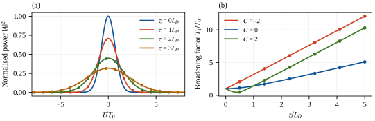
Figure 3(a) shows the evolution of a 25 ps Gaussian pulse (

C = 0

) computed with the SSFM for

z = 0

3 L_{D}

(

L_{D} = 28.8

km). The pulse conserves its Gaussian shape, its peak power drops as

1 / \sqrt{1 + {(z / L_{D})}^{2}}

, and the numerical results are indistinguishable from the analytical envelope (markers). Figure 3(b) shows the broadening factor for three chirp values. A positive chirp (

C = 2

) in the anomalous-dispersion regime first compresses the pulse to a minimum width factor of 0.447 at

z = 0.4 L_{D}

, exactly as predicted by Eq. (19), whereas a negative chirp accelerates the broadening. At

z = 3 L_{D}

(86 km) the unchirped pulse is 3.16 times wider than at the input, which would cause severe inter-symbol interference in a 10 Gb/s system.

Download: Download full-size image

Figure 3. (a) Gaussian pulse evolution in the linear regime (lines: SSFM; markers: analytical envelope). (b) Broadening factor

T_{1} / T_{0}

versus

z / L_{D}

for chirp parameters

C = - 2

, 0 and 2 (lines: Eq. (19); markers: SSFM).

3.3. Self-phase Modulation

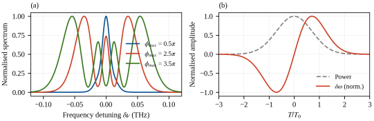
The spectral evolution of a 20 ps Gaussian pulse under pure SPM is presented in Figure 4(a) for three values of the maximum nonlinear phase. The spectrum broadens and develops

M = 1

, 3 and 4 peaks for

ϕ_{\max} = 0.5 π

2.5 π

and

3.5 π

, respectively, which is exactly the number predicted by Eq. (23). The corresponding rms spectral width grows from 9.6 GHz to 54.6 GHz. Figure 4(b) displays the SPM-induced chirp: the leading edge of the pulse is red-shifted and the trailing edge blue-shifted, so that the chirp is approximately linear over the central part of the pulse. In the anomalous-dispersion regime this positive chirp is the key to soliton formation, since it can be compensated by dispersion.

Download: Download full-size image

Figure 4. (a) SPM-broadened spectra of a Gaussian pulse for increasing maximum nonlinear phase. (b) Pulse power and normalized SPM-induced frequency chirp for

ϕ_{\max} = 3.5 π

3.4. Soliton Propagation

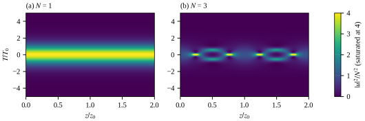
The balance between dispersion and nonlinearity is illustrated in Figure 5. For

N = 1

the sech pulse propagates without any change over two soliton periods; the peak power after

2 z_{0}

is 99.995% of its initial value. For

N = 3

the pulse undergoes a periodic sequence of narrowing, splitting and recombination, with a maximum peak power of

6.15 \times

its initial value around

z = z_{0} / 2

, and recovers its initial shape at

z = z_{0}

. The peak power after

2 z_{0}

is within

2.4 \times 10^{- 4}

(relative) of the initial value, and the pulse energy is conserved to

2 \times 10^{- 12}

. This long-distance fidelity is a stringent test of the scheme, since small splitting errors would accumulate rapidly in such a highly nonlinear regime.

Download: Download full-size image

Figure 5. Evolution of the normalized power

{|U|}^{2} / N^{2}

over two soliton periods for (a) the fundamental soliton (

N = 1

) and (b) the third-order soliton (

N = 3

). The color scale of (b) is saturated at 4.

3.5. Numerical Accuracy and Reach Limits

Figure 6(a) reports the relative

L_{2}

error of the SSFM versus the step size for a second-order soliton (

N = 2

) propagated over

z = π / 4

in normalized units. A linear fit in logarithmic coordinates gives a slope of 1.0 for the asymmetric scheme and 1.9 for the symmetric scheme, confirming the first- and second-order convergence, respectively. For a step of

h = π / (4 \cdot 160)

, the symmetric scheme reaches a relative error of

1.2 \times 10^{- 3}

whereas the asymmetric one gives

1.4 \times 10^{- 2}

; the symmetric scheme thus requires roughly ten times fewer steps for the same accuracy at the cost of one additional FFT pair per step (). Figure 6(b) shows the maximum reach under the dispersion limits of Eq. (31) and

B^{2} L |β_{2}| ≲ 1 / 16

. At 10 Gb/s the reach of an unchirped narrow-linewidth source is about 29 km, and it falls to 1.5 km when the source spectral width is 1 nm.

Download: Download full-size image

Figure 6. (a) Relative

L_{2}

error of the SSFM as a function of the step size for the symmetric and asymmetric schemes (

N = 2

soliton). (b) Dispersion-limited reach as a function of the bit rate for a transform-limited source and for sources with rms spectral widths of 0.1 and 1 nm.

Table 2 summarizes the validation tests. Linear propagation agrees with the analytical solution to machine precision, and all nonlinear benchmarks are reproduced with relative deviations below

10^{- 3}

Table 2. Validation of the numerical model against analytical benchmarks.

Test	Reference value	Simulation	Deviation
Gaussian broadening factor at $z = 3 L_{D}$ ( $C = 0$ )	3.16228	3.16228	$< 10^{- 12}$
Minimum width factor, $C = 2$	0.44721	0.44721	$< 10^{- 8}$
Energy conservation ( $N = 3$ , lossless)	1	1.000000000002	$2 \times 10^{- 12}$
Peak power of $N = 1$ soliton after $2 z_{0}$	1	0.99995	$5 \times 10^{- 5}$
Peak power of $N = 3$ soliton after $2 z_{0}$	9	9.0022	$2.4 \times 10^{- 4}$
SPM spectral peaks for $ϕ_{\max} = 3.5 π$	4	4	–
Convergence order (symmetric / asymmetric)	2 / 1	1.9 / 1.0	–

3.6. Link-level Performance

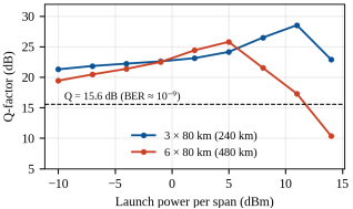
Figure 7 presents the Q-factor of the 2.5 Gb/s NRZ signal as a function of the launch power per span for three and six spans of 80 km. For low launch power the system is limited by ASE noise, and the Q-factor increases with power. Beyond an optimum, SPM-induced waveform distortion combined with chromatic dispersion degrades the signal and Q decreases rapidly. For three spans (240 km) the optimum launch power is +11 dBm with a peak Q of 28.5 dB, whereas for six spans (480 km) the optimum shifts down to +5 dBm and the peak Q decreases to 25.8 dB. The 6 dB shift of the optimum (within the 3 dB resolution of the power grid) for a doubling of the number of spans reflects the accumulation of both noise and nonlinear distortion along the link.

Download: Download full-size image

Figure 7. Q-factor versus launch power per span for a 2.5 Gb/s NRZ signal after three and six 80 km spans. The dashed line marks the Q-factor corresponding to a BER of

10^{- 9}

4. Discussion

The results confirm that a compact scalar model, built on the NLSE and solved by the SSFM, reproduces the principal physical effects governing pulse propagation in single-mode fibers. The dispersion length

L_{D}

and the nonlinear length

L_{NL}

provide a useful guide for anticipating the dominant regime: for the 25 ps pulse considered here,

L_{D} = 28.8

km, so that dispersion dominates over the 80 km span at low power, whereas for launch powers above a few tens of milliwatts the nonlinear length falls below the span length and SPM distorts the waveform. The link simulation shows that the transition between these regimes defines an optimum launch power, a well-known result of nonlinear fiber optics

[4]

. The shift of the optimum towards lower power as the number of spans increases is qualitatively consistent with the accumulation of nonlinear interference in long amplified links.

From a numerical point of view, the comparison with analytical solutions shows that the symmetric SSFM is accurate and efficient. The validation errors of Table 2 are limited only by the temporal discretization for the nonlinear tests and by round-off for the linear test. The observed convergence orders of 1.9 and 1.0 agree with the theoretical values and with previous analyses of step-size selection

[19]

. In practice, the step size must satisfy both the nonlinear-phase criterion of Eq. (27) and a walk-off criterion linked to the bandwidth of the simulation window, otherwise spurious spectral components can appear through aliasing.

The study also shows the limits of the model. First, the scalar NLSE ignores the vector nature of light: in real fibers, polarization-mode dispersion and the Manakov equations should be considered for data rates above 10 Gb/s. Second, for sub-picosecond pulses or operation close to the zero-dispersion wavelength, third-order dispersion, self-steepening and the delayed Raman response become significant

[20, 21]

and must be added to Eq. (15); the split-step framework accommodates these terms with minimal changes. Third, the link model assumes an idealized receiver and a limited number of bits; absolute Q-factor values (up to 28 dB) are therefore optimistic compared with experimental systems, and only the trends should be interpreted. In soliton-based transmission, amplifier noise additionally causes timing jitter, known as the Gordon–Haus effect

[22]

, which is not captured by deterministic simulations.

Natural extensions include multi-channel wavelength-division multiplexing with cross-phase modulation and digital back-propagation. Because the whole solver fits in a few dozen lines of NumPy code, the approach is also well suited to teaching and rapid prototyping.

5. Conclusion

We have presented a complete mathematical model of light propagation in optical fibers, from Maxwell’s equations and guided modes to the nonlinear Schrödinger equation and its numerical solution by the split-step Fourier method. The Python implementation reproduces analytical results for Gaussian pulse broadening, SPM and soliton propagation with errors between

10^{- 12}

and

2.4 \times 10^{- 4}

, and shows the expected second-order convergence of the symmetric scheme. At the system level, a 2.5 Gb/s amplified link exhibits an optimum launch power that decreases from +11 to +5 dBm when the link length doubles from 240 to 480 km. These results provide a validated basis for further studies including polarization effects, Raman scattering and multi-channel transmission.

Abbreviations

CMT	Coupled-Mode Theory
DC	Dual-Core
EM	Electromagnetic
FEM	Finite Element Method
Lc	Coupling Length
LP	Linearly Polarized Mode
MATLAB	Matrix Laboratory
MMF	Multimode Fiber
NA	Numerical Aperture
SNR	Signal-to-Noise Ratio
SMF	Single-Mode Fiber
TE	Transverse Electric
TM	Transverse Magnetic
V	Normalized Frequency
WDM	Wavelength-Division Multiplexing
κ	Coupling Coefficient
$Δn₁₂$	Core-to-Core Refractive-Index Difference
$Δnᶜ$	Core-to-Cladding Refractive-Index Difference

Author Contributions

Randriana Heritiana Nambinina Erica: Conceptualization, Investigation, Methodology, Writing – original draft

Ando Nirina Andriamanalina: Methodology, Supervision, Validation

Conflicts of Interest

The authors declare no conflicts of interest.

References

[1]	K. C. Kao and G. A. Hockham, “Dielectric-fibre surface waveguides for optical frequencies,” Proc. IEE, vol. 113, no. 7, pp. 1151–1158, 1966. https://doi.org/10.1049/piee.1966.0189
[2]	F. P. Kapron, D. B. Keck, and R. D. Maurer, “Radiation losses in glass optical waveguides,” Appl. Phys. Lett., vol. 17, no. 10, pp. 423–425, 1970. https://doi.org/10.1063/1.1653255
[3]	R. J. Mears, L. Reekie, I. M. Jauncey, and D. N. Payne, “Low-noise erbium-doped fibre amplifier operating at 1.54 µm,” Electron. Lett., vol. 23, no. 19, pp. 1026–1028, 1987. https://doi.org/10.1049/el:19870719
[4]	R.-J. Essiambre, G. Kramer, P. J. Winzer, G. J. Foschini, and B. Goebel, “Capacity limits of optical fiber networks,” J. Lightwave Technol., vol. 28, no. 4, pp. 662–701, 2010. https://doi.org/10.1109/JLT.2009.2039464
[5]	G. P. Agrawal, Nonlinear Fiber Optics, 6th ed. Academic Press, 2019. ISBN: 978-0-12-817042-7.
[6]	G. P. Agrawal, Fiber-Optic Communication Systems, 4th ed. Hoboken, NJ, USA: Wiley, 2010. https://doi.org/10.1002/9780470918524
[7]	A. Hasegawa and F. Tappert, “Transmission of stationary nonlinear optical pulses in dispersive dielectric fibers. I. Anomalous dispersion,” Appl. Phys. Lett., vol. 23, no. 3, pp. 142–144, 1973. https://doi.org/10.1063/1.1654836
[8]	L. F. Mollenauer, R. H. Stolen, and J. P. Gordon, “Experimental observation of picosecond pulse narrowing and solitons in optical fibers,” Phys. Rev. Lett., vol. 45, no. 13, pp. 1095–1098, 1980. https://doi.org/10.1103/PhysRevLett.45.1095
[9]	R. H. Hardin and F. D. Tappert, “Applications of the split-step Fourier method to the numerical solution of nonlinear and variable coefficient wave equations,” SIAM Rev. Chronicle, vol. 15, p. 423, 1973.
[10]	A. W. Snyder and J. D. Love, Optical Waveguide Theory. London, U. K.: Chapman and Hall, 1983. https://doi.org/10.1007/978-1-4613-2813-1
[11]	D. Gloge, “Weakly guiding fibers,” Appl. Opt., vol. 10, no. 10, pp. 2252–2258, 1971. https://doi.org/10.1364/AO.10.002252
[12]	I. H. Malitson, “Interspecimen comparison of the refractive index of fused silica,” J. Opt. Soc. Am., vol. 55, no. 10, pp. 1205–1209, 1965. https://doi.org/10.1364/JOSA.55.001205
[13]	ITU-T, “Characteristics of a single-mode optical fibre and cable,” Recommendation G.652, Geneva, Switzerland, 2016.
[14]	G. Keiser, Optical Fiber Communications, 4th ed. New York, NY, USA: McGraw-Hill, 2011.
[15]	R. W. Boyd, Nonlinear Optics, 3rd ed. Burlington, MA, USA: Academic Press, 2008.
[16]	R. H. Stolen and C. Lin, “Self-phase-modulation in silica optical fibers,” Phys. Rev. A, vol. 17, no. 4, pp. 1448–1453, 1978. https://doi.org/10.1103/PhysRevA.17.1448
[17]	V. E. Zakharov and A. B. Shabat, “Exact theory of two-dimensional self-focusing and one-dimensional self-modulation of waves in nonlinear media,” Sov. Phys. JETP, vol. 34, no. 1, pp. 62–69, 1972.
[18]	G. Strang, “On the construction and comparison of difference schemes,” SIAM J. Numer. Anal., vol. 5, no. 3, pp. 506–517, 1968. https://doi.org/10.1137/0705041
[19]	O. V. Sinkin, R. Holzlöhner, J. Zweck, and C. R. Menyuk, “Optimization of the split-step Fourier method in modeling optical-fiber communications systems,” J. Lightwave Technol., vol. 21, no. 1, pp. 61–68, 2003. https://doi.org/10.1109/JLT.2003.808628
[20]	K. J. Blow and D. Wood, “Theoretical description of transient stimulated Raman scattering in optical fibers,” IEEE J. Quantum Electron., vol. 25, no. 12, pp. 2665–2673, 1989. https://doi.org/10.1109/3.40655
[21]	J. M. Dudley, G. Genty, and S. Coen, “Supercontinuum generation in photonic crystal fiber,” Rev. Mod. Phys., vol. 78, no. 4, pp. 1135–1184, 2006. https://doi.org/10.1103/RevModPhys.78.1135
[22]	J. P. Gordon and H. A. Haus, “Random Walk of coherently amplified solitons in optical fiber transmission,” Opt. Lett., vol. 11, no. 10, pp. 665–667, 1986. https://doi.org/10.1364/OL.11.000665

Cite This Article

Plain Text BibTeX RIS

APA Style

Erica, R. H. N., Andriamanalina, A. N. (2026). Mathematical Modelling of Light Propagation in Optical Fibers: From Maxwell’s Equations to Split-Step Simulation of Dispersive and Nonlinear Pulse Dynamics. Science Discovery Mathematics, 1(2), 54-63. https://doi.org/10.11648/j.sdmath.20260102.12

Copy | Download

ACS Style

Erica, R. H. N.; Andriamanalina, A. N. Mathematical Modelling of Light Propagation in Optical Fibers: From Maxwell’s Equations to Split-Step Simulation of Dispersive and Nonlinear Pulse Dynamics. Sci. Discov. Math. 2026, 1(2), 54-63. doi: 10.11648/j.sdmath.20260102.12

Copy | Download

AMA Style

Erica RHN, Andriamanalina AN. Mathematical Modelling of Light Propagation in Optical Fibers: From Maxwell’s Equations to Split-Step Simulation of Dispersive and Nonlinear Pulse Dynamics. Sci Discov Math. 2026;1(2):54-63. doi: 10.11648/j.sdmath.20260102.12

Copy | Download

@article{10.11648/j.sdmath.20260102.12,
  author = {Randriana Heritiana Nambinina Erica and Ando Nirina Andriamanalina},
  title = {Mathematical Modelling of Light Propagation in Optical Fibers: From Maxwell’s Equations to Split-Step Simulation of Dispersive and Nonlinear Pulse Dynamics},
  journal = {Science Discovery Mathematics},
  volume = {1},
  number = {2},
  pages = {54-63},
  doi = {10.11648/j.sdmath.20260102.12},
  url = {https://doi.org/10.11648/j.sdmath.20260102.12},
  eprint = {https://article.sciencepublishinggroup.com/pdf/10.11648.j.sdmath.20260102.12},
  abstract = {Optical fibers carry most of the world’s long-distance data traffic, and reliable mathematical models are essential for designing, optimizing and teaching the systems built on them. This work presents a self-contained mathematical model of light propagation in single-mode optical fibers and its numerical implementation in Python. Starting from Maxwell’s equations, we derive the guided-mode eigenvalue problem of the step-index fiber, the frequency dependence of attenuation and chromatic dispersion from the Sellmeier equation and empirical loss models, and the nonlinear Schrödinger equation (NLSE) governing the slowly varying pulse envelope under the combined effects of loss, dispersion and the Kerr nonlinearity. Closed-form results for Gaussian pulse broadening, self-phase modulation (SPM) and soliton propagation are used as analytical benchmarks and combined with a symmetric split-step Fourier method (SSFM) for the numerical solution. The numerical scheme is validated against these analytical solutions to a relative accuracy better than 10-12 for linear propagation, reproduces the expected number of SPM spectral peaks, preserves fundamental and third-order solitons over two soliton periods, and demonstrates the expected second-order convergence with step size. A link-level simulation of a 2.5 Gb/s amplified system, including amplifier noise, a square-law receiver and the resulting Q-factor, shows an optimum launch power that decreases from approximately +11 dBm to +5 dBm as the number of 80 km spans increases from three to six, illustrating the trade-off between noise accumulation and nonlinear distortion. The results show how a compact, physics-based model, implemented in a few dozen lines of code, reproduces the main performance trade-offs of fiber-optic transmission and provides a validated basis for further studies including polarization effects, Raman scattering and multi-channel transmission.},
 year = {2026}
}

Copy | Download

TY  - JOUR
T1  - Mathematical Modelling of Light Propagation in Optical Fibers: From Maxwell’s Equations to Split-Step Simulation of Dispersive and Nonlinear Pulse Dynamics
AU  - Randriana Heritiana Nambinina Erica
AU  - Ando Nirina Andriamanalina
Y1  - 2026/10/31
PY  - 2026
N1  - https://doi.org/10.11648/j.sdmath.20260102.12
DO  - 10.11648/j.sdmath.20260102.12
T2  - Science Discovery Mathematics
JF  - Science Discovery Mathematics
JO  - Science Discovery Mathematics
SP  - 54
EP  - 63
PB  - Science Publishing Group
SN  - 3142-905X
UR  - https://doi.org/10.11648/j.sdmath.20260102.12
AB  - Optical fibers carry most of the world’s long-distance data traffic, and reliable mathematical models are essential for designing, optimizing and teaching the systems built on them. This work presents a self-contained mathematical model of light propagation in single-mode optical fibers and its numerical implementation in Python. Starting from Maxwell’s equations, we derive the guided-mode eigenvalue problem of the step-index fiber, the frequency dependence of attenuation and chromatic dispersion from the Sellmeier equation and empirical loss models, and the nonlinear Schrödinger equation (NLSE) governing the slowly varying pulse envelope under the combined effects of loss, dispersion and the Kerr nonlinearity. Closed-form results for Gaussian pulse broadening, self-phase modulation (SPM) and soliton propagation are used as analytical benchmarks and combined with a symmetric split-step Fourier method (SSFM) for the numerical solution. The numerical scheme is validated against these analytical solutions to a relative accuracy better than 10-12 for linear propagation, reproduces the expected number of SPM spectral peaks, preserves fundamental and third-order solitons over two soliton periods, and demonstrates the expected second-order convergence with step size. A link-level simulation of a 2.5 Gb/s amplified system, including amplifier noise, a square-law receiver and the resulting Q-factor, shows an optimum launch power that decreases from approximately +11 dBm to +5 dBm as the number of 80 km spans increases from three to six, illustrating the trade-off between noise accumulation and nonlinear distortion. The results show how a compact, physics-based model, implemented in a few dozen lines of code, reproduces the main performance trade-offs of fiber-optic transmission and provides a validated basis for further studies including polarization effects, Raman scattering and multi-channel transmission.
VL  - 1
IS  - 2
ER  -

Copy | Download

Author Information

Randriana Heritiana Nambinina Erica

Telecommunication department, Doctoral School of Engineering Sciences and Innovation (EDSTII), Antananarivo, Madagascar

Biography: Randriana Heritiana Nambinina Erica is a lecturer and researcher at the University of Antananarivo and a faculty member at the École Supérieure Polytechnique d’Antananarivo. He is also a doctoral candidate within the EDSTII doctoral school, specializing in telecommunications. His research focuses primarily on optical fiber technologies, including performance optimization, signal propagation, and applications in high-speed communication systems. He has contributed to several academic and applied research projects related to broadband network development and emerging communication infrastructures in Madagascar. His work reflects a strong commitment to advancing optical communication solutions adapted to local and regional technological needs. He actively participates in scientific activities through teaching, research supervision, and conference contributions.

Research Fields: Telecommunication, transmission, optical fiber, optical communication, Signal Processing

Contact Email

http://orcid.org/0009-0003-8089-172X
Ando Nirina Andriamanalina

Telecommunication department, Doctoral School of Engineering Sciences and Innovation (EDSTII), Antananarivo, Madagascar

Research Fields: Telecommunications, Control Systems, Signal Processing

Contact Email

Download PDF

Submit an Article

Plain Text BibTeX RIS

APA Style

Erica, R. H. N., Andriamanalina, A. N. (2026). Mathematical Modelling of Light Propagation in Optical Fibers: From Maxwell’s Equations to Split-Step Simulation of Dispersive and Nonlinear Pulse Dynamics. Science Discovery Mathematics, 1(2), 54-63. https://doi.org/10.11648/j.sdmath.20260102.12

Copy | Download

ACS Style

Erica, R. H. N.; Andriamanalina, A. N. Mathematical Modelling of Light Propagation in Optical Fibers: From Maxwell’s Equations to Split-Step Simulation of Dispersive and Nonlinear Pulse Dynamics. Sci. Discov. Math. 2026, 1(2), 54-63. doi: 10.11648/j.sdmath.20260102.12

Copy | Download

AMA Style

Erica RHN, Andriamanalina AN. Mathematical Modelling of Light Propagation in Optical Fibers: From Maxwell’s Equations to Split-Step Simulation of Dispersive and Nonlinear Pulse Dynamics. Sci Discov Math. 2026;1(2):54-63. doi: 10.11648/j.sdmath.20260102.12

Copy | Download

@article{10.11648/j.sdmath.20260102.12,
  author = {Randriana Heritiana Nambinina Erica and Ando Nirina Andriamanalina},
  title = {Mathematical Modelling of Light Propagation in Optical Fibers: From Maxwell’s Equations to Split-Step Simulation of Dispersive and Nonlinear Pulse Dynamics},
  journal = {Science Discovery Mathematics},
  volume = {1},
  number = {2},
  pages = {54-63},
  doi = {10.11648/j.sdmath.20260102.12},
  url = {https://doi.org/10.11648/j.sdmath.20260102.12},
  eprint = {https://article.sciencepublishinggroup.com/pdf/10.11648.j.sdmath.20260102.12},
  abstract = {Optical fibers carry most of the world’s long-distance data traffic, and reliable mathematical models are essential for designing, optimizing and teaching the systems built on them. This work presents a self-contained mathematical model of light propagation in single-mode optical fibers and its numerical implementation in Python. Starting from Maxwell’s equations, we derive the guided-mode eigenvalue problem of the step-index fiber, the frequency dependence of attenuation and chromatic dispersion from the Sellmeier equation and empirical loss models, and the nonlinear Schrödinger equation (NLSE) governing the slowly varying pulse envelope under the combined effects of loss, dispersion and the Kerr nonlinearity. Closed-form results for Gaussian pulse broadening, self-phase modulation (SPM) and soliton propagation are used as analytical benchmarks and combined with a symmetric split-step Fourier method (SSFM) for the numerical solution. The numerical scheme is validated against these analytical solutions to a relative accuracy better than 10-12 for linear propagation, reproduces the expected number of SPM spectral peaks, preserves fundamental and third-order solitons over two soliton periods, and demonstrates the expected second-order convergence with step size. A link-level simulation of a 2.5 Gb/s amplified system, including amplifier noise, a square-law receiver and the resulting Q-factor, shows an optimum launch power that decreases from approximately +11 dBm to +5 dBm as the number of 80 km spans increases from three to six, illustrating the trade-off between noise accumulation and nonlinear distortion. The results show how a compact, physics-based model, implemented in a few dozen lines of code, reproduces the main performance trade-offs of fiber-optic transmission and provides a validated basis for further studies including polarization effects, Raman scattering and multi-channel transmission.},
 year = {2026}
}

Copy | Download

TY  - JOUR
T1  - Mathematical Modelling of Light Propagation in Optical Fibers: From Maxwell’s Equations to Split-Step Simulation of Dispersive and Nonlinear Pulse Dynamics
AU  - Randriana Heritiana Nambinina Erica
AU  - Ando Nirina Andriamanalina
Y1  - 2026/10/31
PY  - 2026
N1  - https://doi.org/10.11648/j.sdmath.20260102.12
DO  - 10.11648/j.sdmath.20260102.12
T2  - Science Discovery Mathematics
JF  - Science Discovery Mathematics
JO  - Science Discovery Mathematics
SP  - 54
EP  - 63
PB  - Science Publishing Group
SN  - 3142-905X
UR  - https://doi.org/10.11648/j.sdmath.20260102.12
AB  - Optical fibers carry most of the world’s long-distance data traffic, and reliable mathematical models are essential for designing, optimizing and teaching the systems built on them. This work presents a self-contained mathematical model of light propagation in single-mode optical fibers and its numerical implementation in Python. Starting from Maxwell’s equations, we derive the guided-mode eigenvalue problem of the step-index fiber, the frequency dependence of attenuation and chromatic dispersion from the Sellmeier equation and empirical loss models, and the nonlinear Schrödinger equation (NLSE) governing the slowly varying pulse envelope under the combined effects of loss, dispersion and the Kerr nonlinearity. Closed-form results for Gaussian pulse broadening, self-phase modulation (SPM) and soliton propagation are used as analytical benchmarks and combined with a symmetric split-step Fourier method (SSFM) for the numerical solution. The numerical scheme is validated against these analytical solutions to a relative accuracy better than 10-12 for linear propagation, reproduces the expected number of SPM spectral peaks, preserves fundamental and third-order solitons over two soliton periods, and demonstrates the expected second-order convergence with step size. A link-level simulation of a 2.5 Gb/s amplified system, including amplifier noise, a square-law receiver and the resulting Q-factor, shows an optimum launch power that decreases from approximately +11 dBm to +5 dBm as the number of 80 km spans increases from three to six, illustrating the trade-off between noise accumulation and nonlinear distortion. The results show how a compact, physics-based model, implemented in a few dozen lines of code, reproduces the main performance trade-offs of fiber-optic transmission and provides a validated basis for further studies including polarization effects, Raman scattering and multi-channel transmission.
VL  - 1
IS  - 2
ER  -

Copy | Download