One of the most significant environmental hazards threatening ecosystems is gully erosion. In this study, we applied two bivariate statistical models—frequency ratio (FR) and index of entropy (IoE)—as well as a machine learning algorithm (RF) to generate gully erosion susceptibility maps (GESM). The study was conducted in the Dodota Alem watershed of the Awash River basin, covering 135 km². Our modeling utilized input data from field surveys, Google Earth, and secondary sources. Geo-environmental factors such as land use and land cover, soil characteristics, altitude, slope, aspect, profile curvature, plan curvature, drainage density, distance from roads, distance from streams, stream power index (SPI), and topographic wetness index (TWI) were considered after a multi-collinearity test. Among these factors, distance from roads had the most substantial impact on gully erosion susceptibility according to the RF model, while SPI played a crucial role in the FR and IoE models. Approximately 60% of the watershed falls into the moderate or high susceptibility category for gully erosion using the FR and IoE models, whereas the RF model projected the largest area in the very high susceptibility class. Validation results, based on the Area Under Curve (AUC), demonstrated prediction efficiencies of 0.912 (FR), 0.880 (IoE), and 0.932 (RF). These findings can guide decision-makers and planners in implementing effective soil and water conservation measures to mitigate the damage caused by gully erosion. Additionally, this approach serves as a valuable reference for future research on gully erosion susceptibility.
| Published in | American Journal of Environmental Science and Engineering (Volume 8, Issue 3) |
| DOI | 10.11648/j.ajese.20240803.11 |
| Page(s) | 49-64 |
| Creative Commons |
This is an Open Access article, distributed under the terms of the Creative Commons Attribution 4.0 International License (http://creativecommons.org/licenses/by/4.0/), which permits unrestricted use, distribution and reproduction in any medium or format, provided the original work is properly cited. |
| Copyright |
Copyright © The Author(s), 2024. Published by Science Publishing Group |
Gully Erosion, Machine Learning, Random Forest, Bivariate Models, Ethiopia
Conditional factor | Multi-collinearity | |
|---|---|---|
Tolerance | VIF | |
Altitude | 0.527 | 1.897 |
Aspect | 0.360 | 2.779 |
Profile curvature | 0.353 | 2.834 |
Plan curvature | 0.638 | 1.568 |
Drainage density | 0.337 | 2.963 |
Distance from road | 0.458 | 2.185 |
Distance from stream | 0.375 | 2.669 |
LULC | 0.605 | 1.652 |
Slope | 0.380 | 2.633 |
Soil | 0.565 | 1.770 |
SPI | 0.796 | 1.257 |
TWI | 0.356 | 2.808 |
Factor | Class | Total Pixels | Gully Pixel | FR | ||
|---|---|---|---|---|---|---|
Number | % | Number | % | |||
Altitude | 1527 - 1677 | 304,286 | 35.2 | - | 0.0 | 0.000 |
1678 - 1845 | 334,109 | 38.7 | 1,998 | 16.7 | 0.432 | |
1846 - 2047 | 120,226 | 13.9 | 8,416 | 70.3 | 5.054 | |
2048 - 2293 | 105,529 | 12.2 | 1,554 | 13.0 | 1.063 | |
Aspect | Flat (-1) | 62,051 | 7.8 | 331 | 2.8 | 0.354 |
North (0°to 22.5°) | 112,050 | 14.1 | 1,523 | 12.7 | 0.902 | |
Northeast (22.5° to 67.5°) | 164,951 | 20.8 | 2,660 | 22.2 | 1.071 | |
East (67.5° to 112.5°) | 96,244 | 12.1 | 1,574 | 13.2 | 1.086 | |
Southeast (112.5° to 157.5°) | 59,193 | 7.5 | 482 | 4.0 | 0.541 | |
South (157.5° to 202.5°) | 7,604 | 1.0 | 223 | 1.9 | 1.947 | |
Southwest (202.5° to 247.5°) | 10,149 | 1.3 | 442 | 3.7 | 2.891 | |
West (247.5° to 292.5°) | 81,763 | 10.3 | 1,147 | 9.6 | 0.931 | |
Northwest (292.5° to 337.5°) | 158,914 | 20.0 | 2,700 | 22.6 | 1.128 | |
North (337.5° to 360°) | 41,325 | 5.2 | 881 | 7.4 | 1.415 | |
Profile curvature | -5.8 - -0.6 | 139,907 | 16.2 | 1,974 | 16.7 | 1.034 |
-0.5 - 0 | 162,262 | 18.8 | 2,206 | 18.7 | 0.997 | |
0.1 - 0.6 | 256,892 | 29.7 | 3,438 | 29.2 | 0.981 | |
0.7 - 3.8 | 305,089 | 35.3 | 4,169 | 35.4 | 1.002 | |
Plan curvature | Concave | 10,042 | 1.2 | 260 | 2.2 | 1.870 |
Plan | 844,334 | 97.7 | 11,538 | 96.4 | 0.987 | |
Convex | 9,774 | 1.1 | 165 | 1.4 | 1.219 | |
Drainage density | 0-1 | 263,820 | 30.5 | 3,094 | 25.9 | 0.847 |
1.1-2 | 289,211 | 33.5 | 3,469 | 29.0 | 0.866 | |
2.1-3 | 239,404 | 27.7 | 3,381 | 28.3 | 1.020 | |
3.1-5 | 71,629 | 8.3 | 2,020 | 16.9 | 2.037 | |
Distance from Road | 0 - 630 | 361,326 | 41.8 | 3,643 | 30.9 | 0.739 |
631 - 1443 | 259,563 | 30.0 | 5,714 | 48.5 | 1.614 | |
1444 - 2471 | 149,655 | 17.3 | 2,362 | 20.0 | 1.157 | |
2472 - 4228 | 93,606 | 10.8 | 68 | 0.6 | 0.053 | |
Distance from stream | 0 - 100 | 398,074 | 46.0 | 8,363 | 69.8 | 1.517 |
100 - 200 | 258,492 | 29.9 | 1,965 | 16.4 | 0.549 | |
200 - 300 | 125,907 | 14.6 | 945 | 7.9 | 0.542 | |
300 - 900 | 82,059 | 9.5 | 701 | 5.9 | 0.617 | |
LULC | Settlement | 46,360 | 5.4 | 38 | 0.3 | 0.060 |
Shrubs | 19,956 | 2.3 | 9 | 0.1 | 0.033 | |
Degraded | 37,910 | 4.4 | 1,266 | 10.7 | 2.445 | |
Cultivable | 757,951 | 87.9 | 10,465 | 88.9 | 1.011 | |
Slope | 0 - 5% | 446,883 | 51.8 | 3,109 | 26.8 | 0.517 |
6 - 10% | 325,212 | 37.7 | 5,179 | 44.6 | 1.183 | |
11 - 15% | 65,468 | 7.6 | 2,192 | 18.9 | 2.488 | |
16 - 30% | 24,615 | 2.9 | 1,122 | 9.7 | 3.387 | |
Soil | Eutric fluvisols | 30,857 | 3.6 | - | 0.0 | 0.000 |
Eutric regosols | 649,208 | 75.2 | 4,733 | 40.6 | 0.541 | |
Mollic andosols | 7,796 | 0.9 | 84 | 0.7 | 0.799 | |
Vertic cambisols | 175,985 | 20.4 | 6,833 | 58.7 | 2.879 | |
SPI | 0 - 384 | 859,444 | 99.5 | 11,440 | 98.3 | 0.988 |
385 - 2072 | 4,312 | 0.5 | 164 | 1.4 | 2.823 | |
2073 - 6907 | 365 | 0.0 | 36 | 0.3 | 7.321 | |
6908 - 19571 | 29 | 0.0 | 2 | 0.0 | 5.119 | |
TWI | 3 - 6 | 301,814 | 34.9 | 5,263 | 45.2 | 1.294 |
7 - 8 | 369,035 | 42.7 | 4,264 | 36.6 | 0.858 | |
9 - 10 | 131,715 | 15.2 | 1,336 | 11.5 | 0.753 | |
11 - 19 | 61,586 | 7.1 | 779 | 6.7 | 0.939 | |
Factor | Class | Total Pixels | Gully Pixel | Pij | (Pij) | Hj | Hjmax | Ij | Wj | ||
|---|---|---|---|---|---|---|---|---|---|---|---|
Number | % | Number | % | ||||||||
Altitude | 1527 – 1677 | 304,286 | 35.2 | - | 0.0 | 0.000 | 0.000 | 0.973 | 2.000 | 0.513 | 0.841 |
1678 – 1845 | 334,109 | 38.7 | 1,998 | 16.7 | 0.432 | 0.066 | |||||
1846 – 2047 | 120,226 | 13.9 | 8,416 | 70.3 | 5.054 | 0.772 | |||||
2048 – 2293 | 105,529 | 12.2 | 1,554 | 13.0 | 1.063 | 0.162 | |||||
Aspect | Flat (-1) | 62,051 | 7.8 | 331 | 2.8 | 0.354 | 0.029 | 3.111 | 3.322 | 0.063 | 0.078 |
North (0°to 22.5°) | 112,050 | 14.1 | 1,523 | 12.7 | 0.902 | 0.074 | |||||
Northeast (22.5° to 67.5°) | 164,951 | 20.8 | 2,660 | 22.2 | 1.071 | 0.087 | |||||
East (67.5° to 112.5°) | 96,244 | 12.1 | 1,574 | 13.2 | 1.086 | 0.089 | |||||
Southeast (112.5° to 157.5°) | 59,193 | 7.5 | 482 | 4.0 | 0.541 | 0.044 | |||||
South (157.5° to 202.5°) | 7,604 | 1.0 | 223 | 1.9 | 1.947 | 0.159 | |||||
Southwest (202.5° to 247.5°) | 10,149 | 1.3 | 442 | 3.7 | 2.891 | 0.236 | |||||
West (247.5° to 292.5°) | 81,763 | 10.3 | 1,147 | 9.6 | 0.931 | 0.076 | |||||
Northwest (292.5° to 337.5°) | 158,914 | 20.0 | 2,700 | 22.6 | 1.128 | 0.092 | |||||
North (337.5° to 360°) | 41,325 | 5.2 | 881 | 7.4 | 1.415 | 0.115 | |||||
Profile Curvature | -5.8 - -0.6 | 139,907 | 16.2 | 1,974 | 16.7 | 1.034 | 0.258 | 1.9997 | 2.000 | 0.0001 | 0.0001 |
-0.5 – 0 | 162,262 | 18.8 | 2,206 | 18.7 | 0.997 | 0.248 | |||||
0.1 - 0.6 | 256,892 | 29.7 | 3,438 | 29.2 | 0.981 | 0.244 | |||||
0.7 - 3.8 | 305,089 | 35.3 | 4,169 | 35.4 | 1.002 | 0.250 | |||||
Plan curvature | Concave | 10,042 | 1.2 | 260 | 2.2 | 1.870 | 0.286 | 1.379 | 1.585 | 0.130 | 0.176 |
Plan | 844,334 | 97.7 | 11,538 | 96.4 | 0.987 | 0.151 | |||||
Convex | 9,774 | 1.1 | 165 | 1.4 | 1.219 | 0.186 | |||||
Drainage Density | 0-1 | 263,820 | 30.5 | 3,094 | 25.9 | 0.847 | 0.178 | 1.890 | 2.000 | 0.055 | 0.066 |
1.1-2 | 289,211 | 33.5 | 3,469 | 29.0 | 0.866 | 0.182 | |||||
2.1-3 | 239,404 | 27.7 | 3,381 | 28.3 | 1.020 | 0.214 | |||||
3.1-5 | 71,629 | 8.3 | 2,020 | 16.9 | 2.037 | 0.427 | |||||
Distance from Road | 0 – 630 | 361,326 | 41.8 | 3,643 | 30.9 | 0.739 | 0.207 | 1.606 | 2.000 | 0.197 | 0.176 |
613 – 1443 | 259,563 | 30.0 | 5,714 | 48.5 | 1.614 | 0.453 | |||||
1444 – 2471 | 149,655 | 17.3 | 2,362 | 20.0 | 1.157 | 0.325 | |||||
2472 – 4228 | 93,606 | 10.8 | 68 | 0.6 | 0.053 | 0.015 | |||||
Distance from stream | 0 – 100 | 398,074 | 46.0 | 8,363 | 69.8 | 1.517 | 0.470 | 1.835 | 2.000 | 0.082 | 0.066 |
100 – 200 | 258,492 | 29.9 | 1,965 | 16.4 | 0.549 | 0.170 | |||||
200 – 300 | 125,907 | 14.6 | 945 | 7.9 | 0.542 | 0.168 | |||||
300 – 900 | 82,059 | 9.5 | 701 | 5.9 | 0.617 | 0.191 | |||||
LULC | Settlement | 46,360 | 5.4 | 38 | 0.3 | 0.060 | 0.017 | 1.049 | 2.000 | 0.476 | 0.422 |
Shrubs | 19,956 | 2.3 | 9 | 0.1 | 0.033 | 0.009 | |||||
Degraded | 37,910 | 4.4 | 1,266 | 10.7 | 2.445 | 0.689 | |||||
Cultivated | 757,951 | 87.9 | 10,465 | 88.9 | 1.011 | 0.285 | |||||
Slope | 0 - 5% | 446,883 | 51.8 | 3,109 | 26.8 | 0.517 | 0.068 | 1.730 | 2.000 | 0.135 | 0.256 |
6 - 10% | 325,212 | 37.7 | 5,179 | 44.6 | 1.183 | 0.156 | |||||
11 - 15% | 65,468 | 7.6 | 2,192 | 18.9 | 2.488 | 0.328 | |||||
16 - 30% | 24,615 | 2.9 | 1,122 | 9.7 | 3.387 | 0.447 | |||||
Soil | Eutric fluvisols | 30,857 | 3.6 | - | 0.0 | 0.000 | 0.000 | 1.212 | 2.000 | 0.394 | 0.416 |
Eutric regosols | 649,208 | 75.2 | 4,733 | 40.6 | 0.541 | 0.128 | |||||
Mollic andosols | 7,796 | 0.9 | 84 | 0.7 | 0.799 | 0.189 | |||||
Vertic cambisols | 175,985 | 20.4 | 6,833 | 58.7 | 2.879 | 0.682 | |||||
SPI | 0 – 384 | 859,444 | 99.5 | 11,440 | 98.3 | 0.988 | 0.061 | 1.728 | 2.000 | 0.136 | 0.554 |
385 – 2072 | 4,312 | 0.5 | 164 | 1.4 | 2.823 | 0.174 | |||||
2073 – 6907 | 365 | 0.0 | 36 | 0.3 | 7.321 | 0.450 | |||||
6908 – 19571 | 29 | 0.0 | 2 | 0.0 | 5.119 | 0.315 | |||||
TWI | 3 – 6 | 301,814 | 34.9 | 5,263 | 45.2 | 1.294 | 1.000 | 1.184 | 2.000 | 0.408 | 0.392 |
7 – 8 | 369,035 | 42.7 | 4,264 | 36.6 | 0.858 | 0.663 | |||||
9 – 10 | 131,715 | 15.2 | 1,336 | 11.5 | 0.753 | 0.582 | |||||
11 – 19 | 61,586 | 7.1 | 779 | 6.7 | 0.939 | 0.725 | |||||
Factors | 0 | 1 | MDA | MDG |
|---|---|---|---|---|
Altitude | 4.70 | 4.71 | 4.94 | 0.33 |
Aspect | 4.35 | 4.33 | 4.40 | 0.30 |
Profile curvature | 4.28 | 4.21 | 4.29 | 0.30 |
Plan curvature | -1.00 | -1.00 | -1.00 | 0.05 |
Drainage density | 4.87 | 4.79 | 4.97 | 0.35 |
Distance from road | 4.76 | 4.66 | 4.84 | 0.42 |
Distance from stream | 3.34 | 3.32 | 3.44 | 0.29 |
LULC | 4.40 | 4.39 | 4.56 | 0.39 |
Slope | 4.35 | 4.40 | 4.42 | 0.33 |
Soil | 2.54 | 2.58 | 2.61 | 0.38 |
SPI | 0.73 | 0.00 | 0.49 | 0.03 |
TWI | 4.00 | 3.88 | 4.10 | 0.37 |
Class | FR | IoE | RF | |||
|---|---|---|---|---|---|---|
Area (ha) | Percent | Area (ha) | Percent | Area (ha) | Percent | |
Low | 4562.0 | 34.9 | 4909.2 | 37.5 | 3636.8 | 27.8 |
Moderate | 4237.8 | 32.4 | 4882.0 | 37.3 | 3686.2 | 28.2 |
High | 3284.3 | 25.1 | 2731.5 | 20.9 | 3353.5 | 25.7 |
Very high | 991.3 | 7.6 | 552.6 | 4.2 | 2395.4 | 18.3 |
Total | 13075.3 | 100 | 13075.3 | 100 | 13072.0 | 100 |
| [1] | Amare, S., Langendoen, E., Keesstra, S., van der Ploeg, M., Gelagay, H., Lemma, H., van der Zee, S. E. A. T. M., 2021. Susceptibility to gully erosion: Applying random forest (RF) and frequency ratio (FR) approaches to a small catchment in Ethiopia. Water (Switzerland) 13, 1–22. |
| [2] | Arabameri, A., Blaschke, T., Pradhan, B., Pourghasemi, H. R., Tiefenbacher, J. P., Bui, D. T., 2020a. Evaluation of recent advanced soft computing techniques for gully erosion susceptibility mapping: A comparative study. Sensors (Switzerland) 20, 335–357. |
| [3] | Arabameri, A., Cerda, A., 2019. Spatial Pattern Analysis and Prediction of Gully Erosion Using Novel Hybrid Model of Entropy-Weight of Evidence. Water 11, 1–23. |
| [4] | Arabameri, A., Chen, W., Loche, M., Zhao, X., Li, Y., Lombardo, L., Cerda, A., Pradhan, B., Tien, D., 2020b. Comparison of machine learning models for gully erosion susceptibility mapping Alireza. Geosci. Front. 11, 1609–1620. |
| [5] | Arabameri, A., Rezaei, K., Pourghasemi, H. R., Lee, S., Yamani, M., 2018. GIS-based gully erosion susceptibility mapping: a comparison among three data-driven models and AHP knowledge-based technique. Environ. Earth Sci. 77, 0. |
| [6] | Bajocco, S., De Angelis, A., Perini, L., Ferrara, A., Salvati, L., 2012. The impact of Land Use/Land Cover Changes on land degradation dynamics: A Mediterranean case study. Environ. Manage. 49, 980–989. |
| [7] | Bekele, D., Alamirew, T., Kebede, A., Zeleke, G., M. Melesse, A., 2019. Modeling Climate Change Impact on the Hydrology of Keleta Watershed in the Awash River Basin, Ethiopia. Environ. Model. Assess. 24, 95–107. |
| [8] | Beven, K. J., Kirkby, M. J., 1979. A physically based, variable contributing area model of basin hydrology. Hydrol. Sci. Bull. 24, 43–69. |
| [9] | Borrelli, P., Märker, M., Panagos, P., Schütt, B., 2014. Modeling soil erosion and river sediment yield for an intermountain drainage basin of the Central Apennines, Italy. Catena 114, 45–58. |
| [10] | Breiman, L., 2001. Random forest. Lect. Notes Comput. Sci. (including Subser. Lect. Notes Artif. Intell. Lect. Notes Bioinformatics) 45, 5–32. |
| [11] | Busch, R., Hardt, J., Nir, N., Schütt, B., 2021. Modeling Gully Erosion Susceptibility to Evaluate Human Impact on a Local Modeling Gully Erosion Susceptibility to Evaluate Human Impact on a Local Landscape System in Tigray, Ethiopia. Remote Sens. 13, 2009–2029. |
| [12] | Caté, A., Perozzi, L., Gloaguen, E., Blouin, M., 2017. Machine learning as a tool for geologists. Lead. Edge 64–68. |
| [13] | Chen, W., Li, Y., Xue, W., Shahabi, H., Li, S., Hong, H., Wang, X., Bian, H., Zhang, S., Pradhan, B., Ahmad, B. Bin, 2020. Modeling flood susceptibility using data-driven approaches of naïve Bayes tree, alternating decision tree, and random forest methods. Sci. Total Environ. 701, 134979. |
| [14] | Conforti, M., Aucelli, P. P. C., Robustelli, G., Scarciglia, F., 2011. Geomorphology and GIS analysis for mapping gully erosion susceptibility in the Turbolo stream catchment (Northern Calabria, Italy). Nat. Hazards 56, 881–898. |
| [15] | Conoscenti, C., Agnesi, V., Angileri, S., Cappadonia, C., Rotigliano, E., Märker, M., 2013. A GIS-based approach for gully erosion susceptibility modelling: A test in Sicily, Italy. Environ. Earth Sci. 70, 1179–1195. |
| [16] | Cutler, D. R., Beard, K. H., Cutler, A., Gibson, J., 2007. Random Forests for Classification in Ecology. Ecology 88, 2783–2792. |
| [17] | Devkota, K. C., Regmi, A. D., Pourghasemi, H. R., Yoshida, K., Pradhan, B., Ryu, I. C., Dhital, M. R., Althuwaynee, O. F., 2013. Landslide susceptibility mapping using certainty factor, index of entropy and logistic regression models in GIS and their comparison at Mugling-Narayanghat road section in Nepal Himalaya. Nat. Hazards 65, 135–165. |
| [18] | EMA, 1976. Ethiopian mapping Agency, Topographic Map Series, Addis Ababa, Ethiopia. |
| [19] | Fang, P., Zhang, X., Wei, P., Wang, Y., Zhang, H., Liu, F., Zhao, J., 2020. The classification performance and mechanism of machine learning algorithms in winter wheat mapping using Sentinel-2 10 m resolution imagery. Appl. Sci. 10, 5075–5096. |
| [20] | FAO/UNESCO, 1995. The Digital Soil Map of the World, Food and Agriculture Organization of the United Nations. Rome, Italy. |
| [21] | Gayen, A., Pourghasemi, H. R., Saha, S., Keesstra, S., Bai, S., 2019. Gully erosion susceptibility assessment and management of hazard-prone areas in India using different machine learning algorithms. Sci. Total Environ. 668, 124–138. |
| [22] | Girmay, G., Nyssen, J., Poesen, J., Bauer, H., Merckx, R., Haile, M., Deckers, J., 2012. Land reclamation using reservoir sediments in Tigray, northern Ethiopia. Soil Use Manag. 28, 113–119. |
| [23] | Gómez-Gutiérrez, Á., Conoscenti, C., Angileri, S. E., Rotigliano, E., Schnabel, S., 2015. Using topographical attributes to evaluate gully erosion proneness (susceptibility) in two mediterranean basins: advantages and limitations. Nat. Hazards 79, 291–314. |
| [24] | Guyassa, E., Frankl, A., Zenebe, A., Poesen, J., Nyssen, J., 2018. Gully and soil and water conservation structure densities in semi-arid northern Ethiopia over the last 80 years. Earth Surf. Process. Landforms 43, 1848–1859. |
| [25] | Haregeweyn, N., Poesen, J., Nyssen, J., De Wit, J., Haile, M., Govers, G., Deckers, S., 2006. Reservoirs in Tigray (Northern Ethiopia): characteristics and sediment deposition problems. L. Degrad. Dev. 17, 211–230. |
| [26] | Hosseinalizadeh, M., Kariminejad, N., Chen, W., Pourghasemi, H. R., Alinejad, M., Mohammadian Behbahani, A., Tiefenbacher, J. P., 2019. Gully headcut susceptibility modeling using functional trees, naïve Bayes tree, and random forest models. Geoderma 342, 1–11. |
| [27] | Hurni, H., 1988. Degradation and conservation of the resources in the Ethiopian highlands. Mt. Res. Dev. 8, 123–130. |
| [28] | Ionita, I., Niacsu, L., Petrovici, G., Blebea-Apostu, A. M., 2015. Gully development in eastern Romania: a case study from Falciu Hills. Nat. Hazards 79, 113–138. |
| [29] | Jaafari, A., Najafi, A., Pourghasemi, H. R., Rezaeian, J., Sattarian, A., 2014. GIS-based frequency ratio and index of entropy models for landslide susceptibility assessment in the Caspian forest, northern Iran. Int. J. Environ. Sci. Technol. 11, 909–926. |
| [30] | Jenks, G. F., Caspall, F. C., 1971. Error on choroplethic maps: definition, measurement, reduction. Ann. Assoc. Am. Geogr. 61, 217–244. |
| [31] | Joseph, S., Anitha, K., Srivastava, V. K., Reddy, C. S., Thomas, A. P., Murthy, M. S. R., 2012. Rainfall and Elevation Influence the Local-Scale Distribution of Tree Community in the Southern Region of Western Ghats Biodiversity Hotspot (India). Int. J. For. Res. 2012, 1–10. |
| [32] | Lai, J. S., Tsai, F., 2019. Improving GIS-based landslide susceptibility assessments with multi-temporal remote sensing and machine learning. Sensors (Switzerland) 19, 1–26. |
| [33] | Lawrence, R. L., Wood, S. D., Sheley, R. L., 2006. Mapping invasive plants using hyperspectral imagery and Breiman Cutler classifications (RandomForest). Remote Sens. Environ. 100, 356–362. |
| [34] | Liaw, A., Wiener, M., 2002. Classification and Regression by randomForest. R News 2, 18–22. |
| [35] | Luffman, I. E., Nandi, A., Spiegel, T., 2015. Gully morphology, hillslope erosion, and precipitation characteristics in the Appalachian Valley and Ridge province, southeastern USA. Catena 133, 221–232. |
| [36] | Mekonnen, M., Keesstra, S. D., Baartman, J. E. M., Stroosnijder, L., Maroulis, J., 2017. Reducing Sediment Connectivity Through man-Made and Natural Sediment Sinks in the Minizr Catchment, Northwest Ethiopia. L. Degrad. Dev. 28, 708–717. |
| [37] | Moeini, A., Zarandi, N. K., Pazira, E., Badiollahi, Y., 2015. The relationship between drainage density and soil erosion rate: a study of five watersheds in Ardebil Province, Iran. River Basin Manag. VIII 197, 129–138. |
| [38] | Mohammady, M., Pourghasemi, H. R., Amiri, M., 2019. Land subsidence susceptibility assessment using random forest machine learning algorithm. Environ. Earth Sci. 78, 1–12. |
| [39] | Mohammady, M., Pourghasemi, H. R., Pradhan, B., 2012. Landslide susceptibility mapping at Golestan Province, Iran: A comparison between frequency ratio, Dempster–Shafer, and weights-of-evidence models. J. Asian Earth Sci. 61, 221–236. |
| [40] | Moore, I. D., Grayson, R. B., Ladson, A. R., 1991. Digital terrain modelling: A review of hydrological, geomorphological, and biological applications. Hydrol. Process. 5, 3–30. |
| [41] | Morgan, R. P. C., 2005. Soil Erosion and Conservation, 3rd ed. Blackwell Publishing Ltd, Oxford, UK. |
| [42] | Nyssen, J., Moeyersons, J., Deckers, J., Haile, M., Poesen, J., 2000. Vertic movements and the development of stone covers and gullies, Tigray Highlands, Ethiopia. Zeitschrift für Geomorphol. 44, 145–164. |
| [43] | Nyssen, J., Poesen, J., Moeyersons, J., Haile, M., Deckers, J., 2008. Dynamics of soil erosion rates and controlling factors in the Northern Ethiopian Highlands – towards a sediment budget. Earth Surf. Process. Landforms 33, 695–711. |
| [44] | O’brien, R. M., 2007. A Caution Regarding Rules of Thumb for Variance Inflation Factors. Qual. Quant. 41, 673–690. |
| [45] | Pathak, P., Wani, S. P., Sudi, R. S., 2006. Gully Control in SAT Watersheds. |
| [46] | Peckham, S., 2011. Profile, plan and streamline curvature: a simple derivation and applications, in: Geomorphometry 2011. pp. 27–30. |
| [47] | Pourghasemi, H. R., Yousefi, S., Kornejady, A., Cerdà, A., 2017. Performance assessment of individual and ensemble data-mining techniques for gully erosion modeling. Sci. Total Environ. 609, 764–775. |
| [48] | Rahmati, O., Kalantari, Z., Ferreira, C. S., Chen, W., Soleimanpour, S. M., Kapović-Solomun, M., Seifollahi-Aghmiuni, S., Ghajarnia, N., Kazemi Kazemabady, N., 2022. Contribution of physical and anthropogenic factors to gully erosion initiation. Catena 210, 105925–105936. |
| [49] | Rahmati, O., Tahmasebipour, N., Haghizadeh, A., Pourghasemi, H. R., Feizizadeh, B., 2017. Evaluation of different machine learning models for predicting and mapping the susceptibility of gully erosion. Geomorphology 298, 118–137. |
| [50] | Saha, S., 2017. Groundwater potential mapping using analytical hierarchical process: a study on Md. Bazar Block of Birbhum District, West Bengal. Spat. Inf. Res. 25, 615–626. |
| [51] | Tamene, L., Abera, W., Demissie, B., Desta, G., Woldearegay, K., Mekonnen, K., 2022. Soil erosion assessment in Ethiopia: A review. J. Soil Water Conserv. 77, 144–157. |
| [52] | Tamene, L., Vlek, P. L. G., 2007. Assessing the potential of changing land use for reducing soil erosion and sediment yield of catchments: A case study in the highlands of northern Ethiopia. Soil Use Manag. 23, 82–91. |
| [53] | Trigila, A., Iadanza, C., Esposito, C., Scarascia-Mugnozza, G., 2015. Comparison of Logistic Regression and Random Forests techniques for shallow landslide susceptibility assessment in Giampilieri (NE Sicily, Italy). Geomorphology 249, 119–136. |
| [54] | Valentin, C., Poesen, J., Li, Y., 2005. Gully erosion: Impacts, factors and control. Catena 63, 132–153. |
| [55] | van den Ham, J.-P., 2008. Dodota Spate Irrigation System Ethiopia A case study of. Wageningen university. |
| [56] | Wang, D., Fan, H., Fan, X., 2017. Distributions of recent gullies on hillslopes with different slopes and aspects in the Black Soil Region of Northeast China. Environ. Monit. Assess. 189, 508–523. |
| [57] | Wang, L., Wei, S., Horton, R., Shao, M., 2011. Effects of vegetation and slope aspect on water budget in the hill and gully region of the Loess Plateau of China. Catena 87, 90–100. |
| [58] | Wang, Q., Li, W., Wu, Y., Pei, Y., Xie, P., 2016. Application of statistical index and index of entropy methods to landslide susceptibility assessment in Gongliu (Xinjiang, China). Environ. Earth Sci. 75, 599–612. |
| [59] | Yibeltal, M., Tsunekawa, A., Haregeweyn, N., Adgo, E., Meshesha, D. T., Aklog, D., Masunaga, T., Tsubo, M., Billi, P., Vanmaercke, M., Ebabu, K., Dessie, M., Sultan, D., Liyew, M., 2019. Analysis of long-term gully dynamics in different agro-ecology settings. Catena 179, 160–174. |
| [60] | Zabihi, M., Mirchooli, F., Motevalli, A., Khaledi Darvishan, A., Pourghasemi, H. R., Zakeri, M. A., Sadighi, F., 2018. Spatial modelling of gully erosion in Mazandaran Province, northern Iran. Catena 161, 1–13. |
| [61] | Zeleke, G. and, Hurni, H., 2001. Implications of land use and land cover dynamics for mountain resource degradation in the Northwestern Ethiopian highlands. Mt. Res. Dev. 21, 184–191. |
| [62] |
Zheng, F.-L., 2006. Effect of Vegetation Changes on Soil Erosion on the Loess Plateau1 1Project supported by the Chinese Academy of Sciences (No. KZCX3-SW-422) and the National Natural Science Foundation of China (Nos. 9032001 and 40335050). Pedosphere 16, 420–427.
https://doi.org/https://doi.org/10.1016/S1002-0160(06)60071-4 |
APA Style
Tesfaye, G., Bekele, D., Eshetu, M., Rabo, M., Bezu, A., et al. (2024). Gully Erosion Risk Assessment Using a GIS-Based Bivariate Statistical Models and Machine Learning in the Dodota Alem Watershed, Ethiopia. American Journal of Environmental Science and Engineering, 8(3), 49-64. https://doi.org/10.11648/j.ajese.20240803.11
ACS Style
Tesfaye, G.; Bekele, D.; Eshetu, M.; Rabo, M.; Bezu, A., et al. Gully Erosion Risk Assessment Using a GIS-Based Bivariate Statistical Models and Machine Learning in the Dodota Alem Watershed, Ethiopia. Am. J. Environ. Sci. Eng. 2024, 8(3), 49-64. doi: 10.11648/j.ajese.20240803.11
AMA Style
Tesfaye G, Bekele D, Eshetu M, Rabo M, Bezu A, et al. Gully Erosion Risk Assessment Using a GIS-Based Bivariate Statistical Models and Machine Learning in the Dodota Alem Watershed, Ethiopia. Am J Environ Sci Eng. 2024;8(3):49-64. doi: 10.11648/j.ajese.20240803.11
@article{10.11648/j.ajese.20240803.11,
  author = {Gizaw Tesfaye and Daniel Bekele and Melat Eshetu and Mohamed Rabo and Abebe Bezu and Abera Asefa},
  title = {Gully Erosion Risk Assessment Using a GIS-Based Bivariate Statistical Models and Machine Learning in the Dodota Alem Watershed, Ethiopia
},
  journal = {American Journal of Environmental Science and Engineering},
  volume = {8},
  number = {3},
  pages = {49-64},
  doi = {10.11648/j.ajese.20240803.11},
  url = {https://doi.org/10.11648/j.ajese.20240803.11},
  eprint = {https://article.sciencepublishinggroup.com/pdf/10.11648.j.ajese.20240803.11},
  abstract = {One of the most significant environmental hazards threatening ecosystems is gully erosion. In this study, we applied two bivariate statistical models—frequency ratio (FR) and index of entropy (IoE)—as well as a machine learning algorithm (RF) to generate gully erosion susceptibility maps (GESM). The study was conducted in the Dodota Alem watershed of the Awash River basin, covering 135 km². Our modeling utilized input data from field surveys, Google Earth, and secondary sources. Geo-environmental factors such as land use and land cover, soil characteristics, altitude, slope, aspect, profile curvature, plan curvature, drainage density, distance from roads, distance from streams, stream power index (SPI), and topographic wetness index (TWI) were considered after a multi-collinearity test. Among these factors, distance from roads had the most substantial impact on gully erosion susceptibility according to the RF model, while SPI played a crucial role in the FR and IoE models. Approximately 60% of the watershed falls into the moderate or high susceptibility category for gully erosion using the FR and IoE models, whereas the RF model projected the largest area in the very high susceptibility class. Validation results, based on the Area Under Curve (AUC), demonstrated prediction efficiencies of 0.912 (FR), 0.880 (IoE), and 0.932 (RF). These findings can guide decision-makers and planners in implementing effective soil and water conservation measures to mitigate the damage caused by gully erosion. Additionally, this approach serves as a valuable reference for future research on gully erosion susceptibility.
},
 year = {2024}
}
TY  - JOUR
T1  - Gully Erosion Risk Assessment Using a GIS-Based Bivariate Statistical Models and Machine Learning in the Dodota Alem Watershed, Ethiopia

AU  - Gizaw Tesfaye
AU  - Daniel Bekele
AU  - Melat Eshetu
AU  - Mohamed Rabo
AU  - Abebe Bezu
AU  - Abera Asefa
Y1  - 2024/09/23
PY  - 2024
N1  - https://doi.org/10.11648/j.ajese.20240803.11
DO  - 10.11648/j.ajese.20240803.11
T2  - American Journal of Environmental Science and Engineering
JF  - American Journal of Environmental Science and Engineering
JO  - American Journal of Environmental Science and Engineering
SP  - 49
EP  - 64
PB  - Science Publishing Group
SN  - 2578-7993
UR  - https://doi.org/10.11648/j.ajese.20240803.11
AB  - One of the most significant environmental hazards threatening ecosystems is gully erosion. In this study, we applied two bivariate statistical models—frequency ratio (FR) and index of entropy (IoE)—as well as a machine learning algorithm (RF) to generate gully erosion susceptibility maps (GESM). The study was conducted in the Dodota Alem watershed of the Awash River basin, covering 135 km². Our modeling utilized input data from field surveys, Google Earth, and secondary sources. Geo-environmental factors such as land use and land cover, soil characteristics, altitude, slope, aspect, profile curvature, plan curvature, drainage density, distance from roads, distance from streams, stream power index (SPI), and topographic wetness index (TWI) were considered after a multi-collinearity test. Among these factors, distance from roads had the most substantial impact on gully erosion susceptibility according to the RF model, while SPI played a crucial role in the FR and IoE models. Approximately 60% of the watershed falls into the moderate or high susceptibility category for gully erosion using the FR and IoE models, whereas the RF model projected the largest area in the very high susceptibility class. Validation results, based on the Area Under Curve (AUC), demonstrated prediction efficiencies of 0.912 (FR), 0.880 (IoE), and 0.932 (RF). These findings can guide decision-makers and planners in implementing effective soil and water conservation measures to mitigate the damage caused by gully erosion. Additionally, this approach serves as a valuable reference for future research on gully erosion susceptibility.

VL  - 8
IS  - 3
ER  -
Ethiopian Institute of Agricultural Research (EIAR), Melkassa Agricultural Research Center, Adama, Ethiopia
Ethiopian Institute of Agricultural Research (EIAR), Melkassa Agricultural Research Center, Adama, Ethiopia
Ethiopian Institute of Agricultural Research (EIAR), Melkassa Agricultural Research Center, Adama, Ethiopia
Ethiopian Institute of Agricultural Research (EIAR), Melkassa Agricultural Research Center, Adama, Ethiopia
Ethiopian Institute of Agricultural Research (EIAR), Melkassa Agricultural Research Center, Adama, Ethiopia
Ethiopian Institute of Agricultural Research (EIAR), Melkassa Agricultural Research Center, Adama, Ethiopia
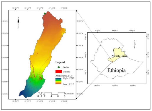
Figure 1. Location and gullies map of Dodota Alem watershed in the Awash Basin.
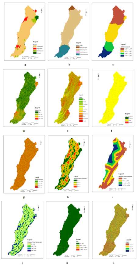
Figure 2. Spatial thematic maps of gully conditioning factors at Dodota Alem watershed: a) land use and land cover (LULC), b) soil type, c) altitude, d) slope, e) aspect f) profile curvature, g) plan curvature, h) drainage density, i) distance from road, j) distance from stream, k) stream power index (SPI) and l) topographic wetness index (TWI).
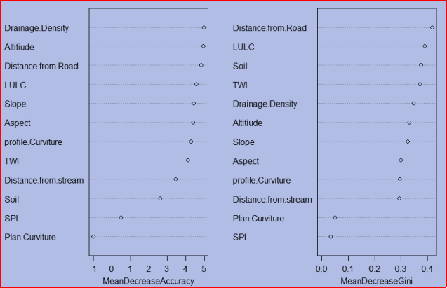
Figure 3. Two measures of variable importance (MDA and MDG) calculated by the random forest algorithm.
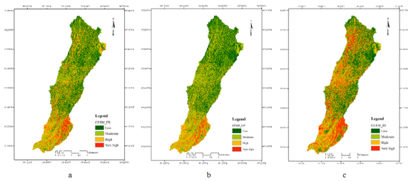
Figure 4. Spatial variability of gully erosion susceptibility using three models at Dodota Alem watershed: a) Frequency ratio, b) Index of entropy, c) Random Forest.
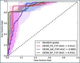
Figure 5. The area under the curve (AUC) of FR, IoE, and RF models.
Information

