A Solar-position-based Analytical Algorithm with Seasonal Atmospheric Correction for Forecasting Bifacial PV Energy Yield in the Fergana Valley

Avazbek Abduraimov; Akmaljon Kuchkarov

doi:doi:10.11648/j.ajme.20261201.13

Research Article |

| Peer-Reviewed

A Solar-position-based Analytical Algorithm with Seasonal Atmospheric Correction for Forecasting Bifacial PV Energy Yield in the Fergana Valley

Avazbek Abduraimov

, Akmaljon Kuchkarov^*

Published in American Journal of Modern Energy (Volume 12, Issue 1)

Received: 11 May 2026 Accepted: 22 May 2026 Published: 5 June 2026

Views: Downloads:

Download PDF

Share This Article

Twitter
Linked In
Facebook

Abstract

Accurate forecasting of photovoltaic energy generation is essential for preliminary system design, seasonal planning and reliable integration of solar power into electric-energy systems. This study proposes a solar-position-based analytical algorithm for estimating the seasonal and annual energy yield of a fixed-tilt bifacial photovoltaic system under the climatic conditions of Fergana city, Uzbekistan. The method combines solar-geometry calculations, monthly atmospheric correction factors, irradiance transposition onto an inclined surface, bifacial rear-side irradiance contribution and NOCT-based module-temperature correction within a unified hourly calculation framework. Monthly atmospheric coefficients were introduced to adapt theoretical clear-sky irradiation to the real seasonal radiation regime of the region. The algorithm was validated against PVsyst simulation results. The proposed method predicted an annual specific yield of 1860 kWh/kWp, while the PVsyst reference value was 1859 kWh/kWp, corresponding to an annual relative deviation of approximately 0.05%. Monthly deviations remained within 5.66%, and the mean absolute percentage error was 2.87%. The results also showed that summer thermal derating may reduce effective PV output by approximately 10–15%, whereas bifacial rear-side generation can increase annual yield by about 5–8%. The proposed algorithm provides a transparent and computationally efficient tool for preliminary photovoltaic energy-yield forecasting in regions with pronounced seasonal climatic variability.

Published in	American Journal of Modern Energy (Volume 12, Issue 1)
DOI	10.11648/j.ajme.20261201.13
Page(s)	9-24
Creative Commons	This is an Open Access article, distributed under the terms of the Creative Commons Attribution 4.0 International License (http://creativecommons.org/licenses/by/4.0/), which permits unrestricted use, distribution and reproduction in any medium or format, provided the original work is properly cited.
Copyright	Copyright © The Author(s), 2026. Published by Science Publishing Group

Keywords

Photovoltaic Energy Forecasting, Solar-position Algorithm, Seasonal Atmospheric Correction, Bifacial Photovoltaic Module, Tilted-plane Irradiance, NOCT Temperature Model, PVsyst Validation, Fergana City

1. Introduction

The increasing penetration of photovoltaic (PV) systems into modern power supply networks has made accurate energy-yield forecasting a critical requirement for system planning, grid operation and investment assessment. Unlike conventional dispatchable generation sources, PV output is governed simultaneously by deterministic astronomical factors and highly variable atmospheric processes. Solar declination, hour angle, zenith angle and panel orientation define the theoretical radiation potential at a given location, whereas cloudiness, aerosol concentration, air temperature and seasonal atmospheric transparency determine the fraction of this potential that is converted into usable irradiance at the module surface. Therefore, a reliable PV forecasting method must account not only for solar geometry, but also for the seasonal variability of local meteorological conditions.

Physics-based irradiance and PV performance models remain widely used because of their transparency, low computational cost and applicability to locations where long historical PV production datasets are unavailable. A key foundation of such models is the accurate determination of the Sun’s apparent position. Reda and Andreas developed the Solar Position Algorithm, which enables high-precision calculation of solar zenith and azimuth angles and has become one of the reference approaches for solar radiation applications

[1]

. However, correct solar-position calculation alone is insufficient for estimating PV energy generation. The global horizontal irradiance must be decomposed into beam and diffuse components, transposed onto the tilted PV plane and corrected for optical, thermal and electrical losses

[2]

. In addition, the treatment of diffuse irradiance is particularly important under partly cloudy conditions, where simplified isotropic models may deviate from more advanced anisotropic transposition approaches such as the Perez model

[3]

Alongside physical models, statistical, machine-learning and hybrid forecasting techniques have been actively developed. Seasonal time-series ensemble approaches have been used to improve operational PV forecasting

[4]

. Recent studies have also introduced decomposition-based deep-learning models

[5]

, machine-learning time-series forecasting approaches

[6]

, PV output-series simulation methods

[7]

, Gaussian process regression for probabilistic short-term forecasting

[8]

, seasonal-trend decomposition combined with optimised recurrent neural networks

[9]

, artificial-intelligence-based irradiance forecasting with uncertainty analysis

[10]

, and quantile deep-learning frameworks for probabilistic PV forecasting

[11]

. These models can provide high predictive performance when sufficient training data and high-quality meteorological inputs are available. Nevertheless, their practical use is often limited in newly developed PV sites, data-scarce regions and preliminary design stages, where measured long-term plant output is unavailable or incomplete.

Another important limitation of many forecasting approaches is their insufficient attention to regional seasonality. In locations with pronounced continental climate, the annual distribution of solar radiation is strongly asymmetric. Summer periods are characterised by higher solar elevation and more stable clear-sky conditions, while winter and transitional months are affected by lower Sun angles and increased cloud occurrence. As a result, forecasting methods based only on annual-average radiation indicators or clear-sky assumptions may systematically overestimate winter production and underestimate the importance of monthly atmospheric correction. This issue is especially relevant for the Fergana Valley of Uzbekistan, where the latitude of approximately 40.4° N and distinct seasonal variability require location-specific correction of theoretical irradiance values

[12]

The growing use of bifacial PV modules introduces an additional modelling requirement. In bifacial PV systems, rear-side generation depends strongly on ground albedo, view factor, rear irradiance distribution and module configuration

[13, 14]

. At the same time, module operating temperature and heat dissipation conditions significantly affect PV energy yield, especially in fixed-tilt and bifacial systems

[15, 16]

Although advanced software packages such as PVsyst allow detailed PV system simulation and performance assessment

[17]

, there remains a practical need for compact analytical algorithms. The suitability of PVsyst as a reference simulation tool is also supported by previous studies evaluating its accuracy in reproducing outdoor PV yield performance

[18]

. Reviews of solar-energy prediction models further show that the choice between physical, statistical and hybrid approaches depends on data availability, forecasting horizon and computational complexity

[19]

The present study addresses this need by developing a solar-position-based analytical algorithm for forecasting the seasonal and annual energy yield of a bifacial photovoltaic system under the climatic conditions of the Fergana Valley. The proposed method combines solar-geometry calculations, decomposition and transposition of irradiance components, monthly atmospheric correction factors, rear-side bifacial gain and NOCT-based temperature derating within a unified hourly calculation framework. The algorithm is then validated against PVsyst simulation results obtained for a representative fixed-tilt bifacial PV installation.

The scientific novelty of this work lies in the integration of three methodological components within a simplified but physically interpretable forecasting framework. First, theoretical solar-position calculations are coupled with month-specific atmospheric correction factors reflecting the seasonal radiation regime of the Fergana Valley. Second, bifacial rear-side irradiance and module-temperature losses are included explicitly rather than treated as constant empirical adjustments. Third, the proposed analytical method is evaluated against PVsyst on both monthly and annual energy-yield scales, allowing the accuracy and limitations of the simplified model to be assessed quantitatively.

2. Materials and Methods

2.1. Study Area and Climatic Background

The proposed photovoltaic energy-yield forecasting algorithm was developed and tested for the climatic conditions of the Fergana Valley, Uzbekistan. The selected region is located at approximately 40.4° N latitude and is characterised by pronounced seasonal variability in solar radiation, ambient temperature and cloudiness. This makes the region suitable for evaluating the influence of solar geometry and month-specific atmospheric correction factors on photovoltaic generation.

The study uses long-term meteorological and solar-radiation characteristics of the region as the climatic basis for seasonal calibration. In particular, monthly average global horizontal irradiance values and cloudiness-related attenuation effects were used to adjust the theoretical clear-sky irradiance obtained from solar-position calculations. The original manuscript identifies the NASA Surface Meteorology and Solar Energy database for the 1983–2005 period and regional meteorological information for the Fergana Valley as the basis for deriving seasonal correction factors.

The need for such correction arises because solar-position models describe the deterministic astronomical component of irradiance, whereas real PV production is also affected by atmospheric transparency, cloud cover, aerosols and seasonal meteorological conditions. Therefore, in this study, the clear-sky theoretical irradiance is not used directly as the final input for PV power estimation; instead, it is modified by monthly atmospheric correction coefficients.

Table 1. Main geographical and climatic input parameters used in the study.

Parameter	Symbol	Value/description	Unit
Study region		Fergana Valley, Uzbekistan
Latitude	φ	≈40.4	degree
Simulation horizon		8760	h
Climatic data basis		Long-term monthly solar-radiation and meteorological data
Main correction type	(K_m)	Monthly atmospheric correction factor
Reference simulation tool		PVsyst

2.2. Photovoltaic System Configuration

The algorithm was applied to a representative fixed-tilt bifacial photovoltaic installation. The selected PV module was a bifacial monocrystalline silicon module with a rated power of 585 Wp. The module surface was oriented with a tilt angle of β = 35° and an azimuth angle of approximately γ = 13° west of south. The ground albedo was taken as ρ = 0.25, representing a moderately reflective ground surface. The nominal operating cell temperature was assumed to be NOCT = 45°C, consistent with typical crystalline-silicon module performance modelling.

The adopted system configuration is summarized in Table 2. These parameters define the geometric, optical and thermal boundary conditions of the analytical calculation. They also ensure that the proposed model and the PVsyst reference simulation are compared under equivalent design assumptions.

Table 2. PV system parameters used in the analytical model and PVsyst validation.

Parameter	Symbol	Value	Unit
Module type		Bifacial monocrystalline silicon
Rated module power	(P_nom)	585	W_p
Tilt angle	β	35	degree
Azimuth angle	γ	≈13 west of south	degree
Ground albedo	ρ	0.25
Nominal operating cell temperature	NOCT	45	°C
Time step	Δt	1	h
Annual simulation period		8760	h

2.3. General Structure of the Forecasting Algorithm

The proposed method is organized as a sequential hourly calculation pipeline. For each hour of the reference year, the model first calculates the solar-position parameters, then estimates extraterrestrial and horizontal irradiance, applies monthly atmospheric correction, separates global radiation into direct and diffuse components, transposes irradiance onto the tilted PV plane, adds the bifacial rear-side contribution, corrects module efficiency for operating temperature and finally integrates hourly power into monthly and annual energy yield.

Download: Download full-size image

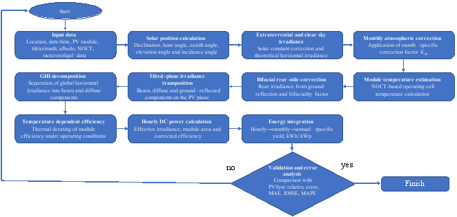
Figure 1. Flowchart of the proposed solar-position-based seasonal PV energy forecasting algorithm.

The calculation sequence is as follows:

1. determination of the day number and local solar time;

2. calculation of solar declination, hour angle, zenith angle and incidence angle;

3. estimation of extraterrestrial irradiance and clear-sky horizontal irradiance;

4. application of monthly atmospheric correction factors;

5. decomposition of global horizontal irradiance into beam and diffuse components;

6. transposition of irradiance from the horizontal plane to the tilted PV plane;

7. estimation of rear-side irradiance for bifacial modules;

8. calculation of module temperature using the NOCT-based approach;

9. correction of PV efficiency for temperature effects;

10. calculation of hourly direct current (DC) power output;

11. aggregation of hourly values into monthly and annual energy yield;

12. validation against PVsyst simulation outputs.

This structure was selected because it preserves the physical transparency of the calculation while requiring fewer input data than advanced machine-learning or numerical weather prediction approaches.

2.4. Analytical Modelling Procedure for Solar Irradiance and PV Energy Yield

The first stage of the algorithm determines the Sun’s apparent position for each hourly time step. The extraterrestrial irradiance normal to the solar beam is calculated as:

G_{on} = G_{sc} [1 + 0.033 \cos (\frac{360 n}{365})]

where, G_sc = 1367 Wm^-2 is the solar constant and n is the day number of the year.

The solar declination angle is determined by:

δ = 23.45 \sin [\frac{360 (284 + n)}{365}]

where, δ is expressed in degrees.

The hour angle is calculated as:

ω = 15 (t_{s} - 12)

where, t_s is the local solar time in decimal hours.

The solar zenith angle is obtained from:

\cos θ_{z} = \sin φ \sin δ + \cos φ \cos δ \cos ω

where, φ is the site latitude.

The solar elevation angle is then:

α_{s} = 90 ° - θ_{z}

For a tilted PV surface, the angle of incidence between the direct solar beam and the module plane is calculated by:

\cos θ_{i} = \sin δ \sin φ \cos β - \sin δ \cos φ \sin β \cos γ + \cos δ \cos φ \cos β \cos ω + \cos δ \sin φ \sin β \cos γ \cos ω + \cos δ \sin β \sin γ \sin ω

here, β is the module tilt angle and γ is the surface azimuth angle. This formulation allows the model to account for the effect of both tilt and azimuth on the incident beam irradiance

[1]

Estimation and decomposition of global horizontal irradiance

The extraterrestrial horizontal irradiance is calculated as:

G_{0 h} = G_{on} \cos θ_{z}

For daylight hours, the clearness index is defined as:

K_{t} = \frac{G_{h}}{G_{0 h}}

where G_h is the global horizontal irradiance after atmospheric correction.

To separate the global horizontal irradiance into beam and diffuse components, the Erbs-type diffuse fraction correlation may be used. PVsyst documentation also identifies the Erbs model as a simple and effective clearness-index-based approach for estimating the diffuse horizontal irradiance fraction from global horizontal irradiance

[2]

The diffuse fraction is expressed as:

\frac{G_{d}}{G_{h}} = \{\begin{matrix} 1 - 0.09 K_{t}, K_{t} \leq 0.22 \\ 0.9511 - 0.1604 K_{t} + 4.388 K_{t}^{2} - 16.638 K_{t}^{3} + 12.336 K_{t}^{4}, 0.22 < K_{t} < 0.80 \\ 0.165, K_{t} > 0.80 \end{matrix}

Then:

G_{d} = G_{h} (\frac{G_{d}}{G_{h}})

and the beam horizontal component is calculated as:

G_{b} = G_{h} = G_{d}

This decomposition is required because beam, diffuse and reflected radiation interact differently with a tilted PV surface.

Transposition of irradiance onto the tilted PV plane

The total front-side irradiance incident on the tilted PV plane is calculated as the sum of beam, diffuse and ground-reflected components:

G_{POA} = G_{b, t} + G_{d, t} + G_{r, t}

The beam component on the tilted plane is:

G_{b, t} = G_{b} R_{b}

where the beam tilt factor is:

R_{b} = \frac{\cos θ_{i}}{\cos θ_{z}}

The diffuse component is estimated using the isotropic sky approximation:

G_{d, t} = G_{d} (\frac{1 + \cos β}{2})

The ground-reflected component is calculated as:

G_{r, t} = G_{h} ρ (\frac{1 - \cos β}{2})

Thus, the total plane-of-array irradiance becomes:

G_{POA} = G_{b} R_{b} + G_{d} (\frac{1 + \cos β}{2}) + G_{h} ρ (\frac{1 - \cos β}{2})

The isotropic diffuse model was selected to keep the algorithm analytically simple and suitable for preliminary engineering calculations

[3]

. However, this simplification is also a source of uncertainty, especially under partly cloudy conditions. More advanced transposition models, such as the Perez model, are commonly used for estimating plane-of-array irradiance from horizontal irradiance data; Sandia PVPMC describes the Perez model as a widely used approach for tilted-plane irradiance estimation, while PVsyst documentation notes that PVsyst provides Hay-Davies and Perez transposition options

[17]

For this reason, the selected PVsyst transposition model must be explicitly reported in the validation setup.

Monthly atmospheric correction

The key methodological feature of the present algorithm is the introduction of monthly atmospheric correction factors. These coefficients account for the difference between theoretical clear-sky irradiance and the long-term monthly solar-radiation regime of the Fergana Valley.

For each month m, the corrected global horizontal irradiance is defined as:

G_{h, m}^{corr} (t) = K_{m} G_{h}^{clear} (t)

where

G_{h}^{clear} (t)

is the theoretical clear-sky horizontal irradiance obtained from solar-position calculations and Km is the monthly atmospheric correction factor.

The monthly correction factor is determined as:

K_{m} = \frac{{\overset{̅}{H}}_{m}^{obs}}{{\overset{̅}{H}}_{m}^{clear}}

where

{\overset{̅}{H}}_{m}^{obs}

is the long-term observed or database-derived monthly mean daily global horizontal irradiation and

{\overset{̅}{H}}_{m}^{clear}

is the corresponding clear-sky monthly mean daily irradiation calculated by the solar-position model.

This approach allows the model to retain the deterministic astronomical structure of solar radiation while correcting its magnitude according to the regional seasonal atmospheric conditions. Winter months are expected to have lower correction factors because of lower solar elevation and increased cloudiness, whereas summer months are expected to approach clear-sky conditions more closely.

For the Fergana city case study, monthly atmospheric correction factors were calculated as the ratio between the observed or database-derived monthly mean daily global horizontal irradiation and the theoretical clear-sky irradiation obtained from solar-geometry calculations. The geographical coordinates of Fergana city were taken as approximately 40.384° N latitude and 71.784° E longitude. The correction coefficient Km therefore represents the combined seasonal influence of cloudiness, atmospheric transparency, aerosol loading and regional climatic attenuation on the available solar radiation.

Table 3. Monthly atmospheric correction factors used in the proposed algorithm.

Month	Clear-sky irradiation, ${\overset{̅}{H}}_{m}^{clear}$ , kWh/m²·day	Observed/database irradiation, ${\overset{̅}{H}}_{m}^{obs}$ , kWh/m²·day	Correction factor, (K_m)
January	4.09	2.25	0.550
February	5.58	2.83	0.507
March	7.50	3.28	0.437
April	9.59	4.19	0.437
May	11.02	5.45	0.495
June	11.63	6.71	0.577
July	11.34	6.84	0.603
August	10.18	6.82	0.670
September	8.29	6.03	0.728
October	6.20	3.90	0.629
November	4.46	2.49	0.559
December	3.70	1.98	0.535

The obtained correction factors indicate a pronounced seasonal variation in atmospheric attenuation. The lowest values were obtained in March–April, where transitional cloudiness and atmospheric instability reduce the effective radiation relative to the theoretical clear-sky potential. Higher correction factors in August–September indicate more favorable atmospheric transparency and stable solar conditions. Therefore, the use of a single annual correction coefficient would be insufficient for reliable seasonal PV energy-yield forecasting in the Fergana region.

Bifacial rear-side irradiance model

For bifacial PV modules, the rear side contributes additional energy yield by absorbing radiation reflected from the ground. in the proposed simplified model, the rear-side irradiance is estimated as:

G_{rear} = ρ G_{h} F_{v}

where ρ is the ground albedo and Fv is the rear-side view factor between the module and the ground surface.

The effective irradiance available for bifacial power generation is then calculated as:

G_{eff} = G_{POA} + η_{rear} G_{rear}

where η_rear is the bifaciality factor, defined as the ratio of rear-side to front-side efficiency.

This simplified treatment is suitable for preliminary energy-yield forecasting, but it does not resolve rear-side irradiance non-uniformity, row-to-row shading or detailed ground-reflection geometry. recent bifacial PV studies show that rear-side irradiance modelling depends strongly on albedo, view-factor assumptions and system geometry

[13, 14]

; therefore, more detailed view-factor or ray-tracing models may be required for final engineering design

[20]

Module temperature and efficiency correction

The operating temperature of the PV module was estimated using a NOCT-based empirical model:

T_{c} = T_{a} + (\frac{NOCT - 20}{800}) G_{eff}

where Tc is the cell temperature, Ta is the ambient air temperature and Geff is the effective irradiance incident on the module surface.

The NOCT approach is widely used because it requires only ambient temperature, irradiance and the manufacturer-reported NOCT value. According to the PV module temperature modelling literature, the NOCT/Ross formulation is one of the simplest explicit approaches for estimating module operating temperature, with the standard NOCT reference conditions commonly associated with 800 W/m² irradiance, 20°C ambient temperature, 1 m/s wind speed and open-rack mounting conditions

[21, 22]

. Previous studies have shown that module temperature and heat dissipation conditions significantly influence PV energy yield

[15, 16]

The temperature-dependent module efficiency is calculated as:

η (T_{s}) = η_{ref} [1 + γ (T_{c} - 25)]

where ηref is the module efficiency under Standard Test Conditions and γ is the temperature coefficient of power. For crystalline-silicon modules, γ is negative; therefore, an increase in cell temperature reduces module efficiency.

This correction is necessary because high summer irradiance increases potential generation, but simultaneously raises cell temperature and causes thermal derating. Without temperature correction, summer energy production would be systematically overestimated.

Electrical power and energy-yield calculation

For the purpose of annual and monthly energy-yield forecasting, the instantaneous DC power output per unit installed capacity is calculated using an efficiency-based model:

P_{DC} (t) = G_{eff} (t) A_{m} η (T_{c})

where A_m is the active module area.

For normalized energy-yield analysis, the output can be expressed per unit installed peak power:

Y (t) = \frac{P_{DC} (t)}{P_{nom}}

Hourly energy production is then calculated as:

E_{h} = P_{DC} (t) ∆ t

where Δt = 1 h.

Monthly energy yield is obtained by summing hourly values within each month:

E_{m} = \sum_{t = 1}^{N_{m}} E_{h} (t)

where N_m is the number of hourly time steps in month m.

Annual energy yield is calculated as:

E_{year} = \sum_{m = 1}^{12} E_{m}

The specific annual yield is expressed as:

Y_{f} = \frac{E_{year}}{P_{nom}}

with units of kWh/kWp.

In this revised methodology, the single-diode equation is not used as the primary computational basis for annual energy-yield forecasting. This is intentional. The study aims to develop a transparent seasonal energy-yield algorithm rather than a detailed I–V curve model. If the single-diode model is retained in the manuscript, then diode saturation current, series resistance, shunt resistance, ideality factor and maximum power point extraction procedure must also be reported. Otherwise, the efficiency-based DC power model is more consistent with the declared scope of the paper.

2.5. PVsyst Reference Simulation

PVsyst was used as the reference engineering simulation environment because it provides established procedures for PV performance assessment, irradiance transposition and loss modelling

[17]

. Its use as a validation reference is supported by previous studies assessing PVsyst simulation accuracy under outdoor operating conditions

[18]

For reproducibility, the PVsyst simulation setup must report the following parameters.

Table 4. PVsyst reference simulation settings.

Parameter	Value / setting
Location	Fergana Valley, Uzbekistan
Latitude	≈40.4° N
Module type	Bifacial monocrystalline silicon
Rated module power	585 Wp
Tilt angle	35°
Azimuth angle	≈13° west of south
Ground albedo	0.25
Meteorological dataset	NASA Surface Meteorology and Solar Energy database, 1983–2005
Transposition model	Perez anisotropic transposition model
Thermal model	NOCT-based module-temperature model; NOCT = 45°C
Simulation time step	Hourly
Output indicators	Monthly and annual specific yield, kWh/kWp

The annual yield predicted by the proposed algorithm was compared with the annual specific yield obtained from PVsyst. In the original manuscript, the proposed model gives approximately 1860 kWh/kWp, while the PVsyst reference value is 1859 kWh/kWp. However, to make the validation scientifically stronger, annual agreement alone is insufficient. Monthly comparison and error metrics must also be reported.

2.6. Validation Metrics and Error Analysis

To quantify the agreement between the proposed analytical algorithm and PVsyst, the following deterministic error metrics were used. Solar forecasting studies commonly apply MAE, MBE, RMSE and related normalized indicators to evaluate forecasting accuracy across different time scales

[23]

The mean bias error is:

MBE = \frac{1}{N} \sum_{i = 1}^{N} (E_{model, i} - E_{ref, i})

where E_model,i is the monthly energy yield predicted by the proposed algorithm and E_ref,i is the corresponding PVsyst reference value.

The mean absolute error is:

MAE = \frac{1}{N} \sum_{i = 1}^{N} |E_{model, i} - E_{ref, i}|

The root mean square error is:

RMSE = \sqrt{\frac{1}{N} \sum_{i = 1}^{N} {(E_{model, i} - E_{ref, i})}^{2}}

The mean absolute percentage error is:

MAPE = \frac{100}{N} \sum_{i = 1}^{N} |\frac{E_{model, i} - E_{ref, i}}{E_{ref, i}}|

The relative monthly deviation is calculated as:

ε_{i} = \frac{E_{model, i} - E_{ref, i}}{E_{ref, i}} \times 100 %

The annual relative deviation is:

ε_{year} = \frac{E_{model}^{year} - E_{year}^{ref}}{E_{year}^{ref}} \times 100 %

Table 5. Monthly validation of the proposed algorithm against PVsyst.

Month	Proposed algorithm, kWh/kWp	PVsyst, kWh/kWp	Absolute error, kWh/kWp	Relative error,%
January	81	84	3	-3.57
February	99	101	2	-1.98
March	141	134	7	+5.22
April	164	160	4	+2.50
May	194	191	3	+1.57
June	211	214	3	-1.40
July	220	224	4	-1.79
August	216	220	4	-1.82
September	199	198	1	+0.51
October	168	159	9	+5.66
November	96	99	3	-3.03
December	71	75	4	-5.33
Annual	1860	1859	1	+0.05

The monthly validation results demonstrate that the proposed analytical algorithm reproduces the PVsyst reference simulation with acceptable accuracy over the entire annual cycle. The annual specific yield estimated by the proposed method was 1860 kWh/kWp, while the PVsyst reference value was 1859 kWh/kWp, corresponding to an annual relative deviation of only 0.05%. Monthly deviations remained within the range of approximately 0.5–5.7%. The highest discrepancies were observed in March and October, which may be attributed to increased variability of atmospheric transparency and cloudiness during transitional seasons. This confirms that the proposed seasonal correction approach is suitable for preliminary engineering assessment, although higher-resolution meteorological data would be required for more precise short-term forecasting.

Table 6. Summary of validation error metrics.

Metric	Value
MBE, kWh/kWp	0.08
MAE, kWh/kWp	3.92
RMSE, kWh/kWp	4.43
MAPE,%	2.87
Maximum monthly relative error,%	5.66
Annual relative deviation,%	0.05

Assumptions and model limitations

The proposed method is intended for preliminary engineering assessment and seasonal energy-yield forecasting. Therefore, several simplifying assumptions were adopted.

First, the diffuse component was calculated using an isotropic sky approximation. This makes the model computationally simple but may introduce errors under partly cloudy conditions, especially during transitional months. Second, the monthly atmospheric correction factors represent average seasonal behavior and do not reproduce stochastic daily weather fluctuations. Third, the bifacial rear-side irradiance model uses a simplified albedo-view-factor approach and does not explicitly resolve rear-side irradiance non-uniformity, row spacing, module elevation or shading effects. Fourth, the NOCT-based temperature model provides an approximate estimate of module temperature and does not explicitly include wind speed or mounting-specific convective heat transfer.

Despite these limitations, the model is suitable for rapid estimation of annual and monthly PV energy yield when detailed measured production data are unavailable. Its main advantage is that each calculation step has a clear physical meaning and can be independently checked, adjusted or replaced by a more detailed sub-model if higher accuracy is required.

3. Results and Discussions

The proposed solar-position-based seasonal forecasting algorithm was applied to the Fergana city case study over a complete annual simulation period using an hourly calculation step. The obtained results demonstrate that photovoltaic energy generation in the studied region is governed by a pronounced seasonal structure resulting from the combined influence of solar geometry, atmospheric transparency, module temperature and bifacial rear-side irradiance. The calculated annual global horizontal irradiation was approximately 1736 kWh/m², indicating a favorable solar-energy potential for photovoltaic applications; however, its monthly distribution was highly non-uniform. During the summer period, particularly in June–August, high solar elevation, longer daylight duration and relatively stable atmospheric conditions produced the highest radiation levels, with July daily irradiation reaching approximately 7–8 kWh/m²·day. In contrast, winter months showed substantially lower irradiation because of reduced solar altitude, shorter daylight duration and increased atmospheric attenuation, with January values decreasing to approximately 2–3 kWh/m²·day

[12]

Download: Download full-size image

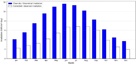
Figure 2. Monthly clear-sky and corrected irradiation for Fergana city.

Figure 2 compares the theoretical clear-sky irradiation with the corrected irradiation values for the Fergana city case study. The difference between the two datasets demonstrates the effect of seasonal atmospheric attenuation and confirms the need for monthly correction factors in solar-position-based PV energy-yield forecasting. This seasonal contrast confirms that annual-average radiation indicators alone are insufficient for reliable PV energy-yield forecasting in the Fergana region. The use of monthly atmospheric correction factors improved the physical realism of the model by adapting the theoretical clear-sky radiation curve to the actual seasonal radiation regime. The correction coefficients reported in Table 3 varied considerably throughout the year, with the lowest values occurring in March and April and the highest value in September, showing that atmospheric attenuation cannot be represented by a constant annual coefficient.

Download: Download full-size image

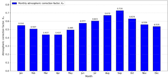
Figure 3. Monthly atmospheric correction factors for the Fergana city case study.

Figure 3 illustrates the monthly atmospheric correction factor K_m for the Fergana city case study. The results show that atmospheric attenuation varies substantially during the year and cannot be represented by a single annual coefficient. The lowest values were observed in March and April, while the highest value was obtained in September, confirming the importance of seasonal correction in solar-position-based PV energy-yield forecasting. After the corrected irradiance was transposed onto the tilted PV plane and adjusted for bifacial rear-side contribution and NOCT-based thermal effects, the predicted monthly PV energy yield followed the expected seasonal pattern. The highest specific yield was obtained in July, reaching approximately 220 kWh/kWp, while June and August also exceeded 210 kWh/kWp. The lowest monthly yield was obtained in December, at approximately 71 kWh/kWp.

Download: Download full-size image

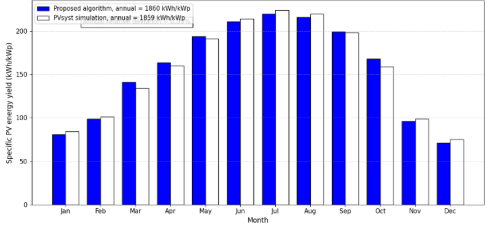
Figure 4. Monthly specific PV energy yield predicted by the proposed analytical algorithm and simulated in PVsyst for the Fergana city case study.

Figure 4 compares the monthly specific PV energy yield predicted by the proposed analytical algorithm with the corresponding PVsyst simulation results. The close agreement between the two datasets confirms that the proposed method can reproduce the seasonal distribution of PV generation with acceptable accuracy. The use of PVsyst as the reference simulation environment is justified by its established engineering modelling framework

[17]

and by previous studies evaluating its accuracy in reproducing outdoor PV yield performance

[18]

. The largest deviations occur in transitional months, where atmospheric variability and diffuse-radiation uncertainty are more pronounced. The proposed algorithm predicted an annual specific yield of 1860 kWh/kWp, while the PVsyst reference simulation gave 1859 kWh/kWp, corresponding to an annual absolute difference of only 1 kWh/kWp and a relative deviation of approximately 0.05%. Since annual agreement alone may conceal compensating monthly errors, the monthly validation results in Table 5 were also analysed. The maximum positive deviations occurred in March and October, reaching approximately +5.22% and +5.66%, respectively, while the largest negative deviation was observed in December, at approximately −5.33%. These discrepancies are physically reasonable because transitional months are characterised by higher variability in cloudiness, diffuse-radiation fraction and atmospheric transparency.

Download: Download full-size image

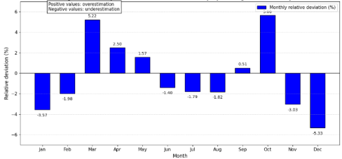
Figure 5. Monthly relative deviation between the proposed analytical algorithm and PVsyst for the Fergana city case study.

Figure 5 presents the monthly relative deviation between the proposed analytical algorithm and the PVsyst reference simulation. The results show that the monthly deviations remain within an acceptable range, with the highest positive deviations observed in March and October and the largest negative deviation observed in December. This pattern confirms that the main discrepancies occur during transitional months, when atmospheric variability and diffuse-radiation uncertainty are more pronounced.

The use of several validation indicators is consistent with recommended practice in solar-power forecasting assessment, where a single metric may not fully describe model performance across seasonal time scales

[23]

. The error metrics reported in Table 6 further confirm the reliability of the proposed method: the mean absolute error was 3.92 kWh/kWp, the root mean square error was 4.43 kWh/kWp, and the mean absolute percentage error was 2.87%. The mean bias error was close to zero, indicating that the model does not have a significant systematic tendency to overestimate or underestimate monthly PV generation. Figure 6 summarizes the validation error metrics of the proposed analytical algorithm. The MAE and RMSE values indicate that the absolute monthly deviations remain moderate, while the MAPE value confirms acceptable monthly-scale accuracy.

Download: Download full-size image

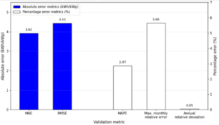
Figure 6. Summary of validation error metrics for the proposed analytical algorithm compared with the PVsyst reference simulation.

The very low annual relative deviation shows that the proposed method reproduces the annual PV energy yield with high agreement relative to the PVsyst reference simulation. The temperature-correction component had a noticeable effect during the summer months. Although June, July and August provided the highest irradiance levels, elevated module temperature reduced the electrical conversion efficiency; according to the model assumptions, the thermal derating effect may reach approximately 10–15% relative to Standard Test Conditions.

Download: Download full-size image

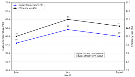
Figure 7. Estimated influence of module temperature on PV performance during summer months for the Fergana city case study.

Figure 7 illustrates the estimated influence of module temperature on PV performance during the summer months. The results show that although solar radiation is highest in June–August, the operating temperature of the module also rises significantly, causing thermal derating of electrical efficiency. This behavior is consistent with previous studies showing that module temperature and heat dissipation conditions significantly influence PV energy yield

[15, 16, 22]

. This confirms that irradiance-only forecasting would overestimate summer energy generation unless module-temperature effects are explicitly included. The bifacial correction also increased the estimated annual yield compared with a monofacial equivalent. For the adopted ground albedo of ρ = 0.25, the rear-side contribution increased annual generation by approximately 5–8%, confirming that bifacial gain should not be ignored in annual PV yield assessment.

Figure 8 compares the annual specific energy yield of the bifacial PV configuration with a monofacial equivalent. The results show that rear-side irradiance increases the annual yield by approximately 6.5%, which falls within the estimated 5–8% bifacial gain range. This confirms that rear-side generation should be included in annual PV energy-yield forecasting, especially when bifacial modules are used. The obtained bifacial gain is physically reasonable because rear-side generation is governed by albedo, rear irradiance distribution, view factor and system geometry

[13, 14]

Download: Download full-size image

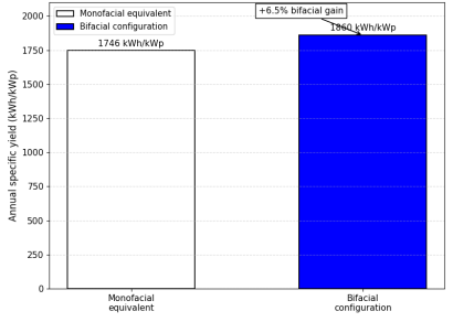
Figure 8. Contribution of bifacial rear-side generation to annual PV energy yield for the Fergana city case study.

Overall, the results show that the proposed algorithm provides an engineering-grade approximation of PV energy generation for the Fergana city case study by combining deterministic solar-position calculations, monthly atmospheric correction, tilted-plane irradiance transposition, bifacial rear-side gain and NOCT-based thermal derating. The remaining deviations relative to PVsyst are mainly associated with simplified diffuse-radiation modelling and the use of monthly average atmospheric correction factors rather than fully stochastic hourly meteorological sequences; therefore, further improvement should focus on higher-resolution atmospheric inputs, more advanced diffuse-radiation transposition and detailed bifacial irradiance modelling. The remaining deviations relative to PVsyst are mainly associated with simplified diffuse-radiation modelling

[3]

, clearness-index-based decomposition

[2]

, simplified rear-side bifacial representation

[13, 14]

, empirical module-temperature estimation

[21, 22]

, and the difference between the proposed analytical model and the detailed PVsyst simulation framework

[17]

4. Conclusions

This study developed and validated a solar-position-based analytical algorithm for forecasting the seasonal and annual energy yield of a bifacial photovoltaic system under the climatic conditions of Fergana city, Uzbekistan. The proposed approach integrates deterministic solar-geometry calculations, monthly atmospheric correction factors, tilted-plane irradiance transposition, bifacial rear-side irradiance contribution and NOCT-based module-temperature correction within a unified hourly calculation framework. Unlike purely clear-sky or annual-average estimation methods, the algorithm accounts for the pronounced seasonal variability of atmospheric transparency, which is essential for reliable photovoltaic generation assessment in continental climate regions.

The results confirmed that the solar-resource availability in the Fergana city case study has a strongly non-uniform annual distribution. The annual global horizontal irradiation was estimated at approximately 1736 kWh/m², while monthly solar availability varied substantially between winter and summer periods. The use of monthly atmospheric correction factors made it possible to adapt theoretical clear-sky irradiation to the realistic regional radiation regime. This correction was particularly important during transitional months, where cloudiness and atmospheric instability caused larger deviations from the ideal solar-geometry-based radiation curve.

Validation against the PVsyst reference simulation demonstrated that the proposed analytical model can reproduce annual photovoltaic energy yield with high accuracy. The annual specific yield predicted by the proposed algorithm was 1860 kWh/kWp, compared with 1859 kWh/kWp obtained from PVsyst, corresponding to an annual relative deviation of approximately 0.05%. At the monthly scale, the maximum relative deviation remained below 5.66%, while the calculated MAPE was 2.87%. These indicators confirm that the model provides sufficient accuracy for preliminary engineering assessment, seasonal planning and early-stage photovoltaic system design.

The results also showed that module-temperature correction and bifacial rear-side generation are not negligible in annual PV yield forecasting. Elevated summer module temperatures may reduce effective power output by approximately 10–15% relative to Standard Test Conditions, meaning that irradiance-only models may overestimate summer generation. At the same time, bifacial rear-side irradiance increased the annual yield by approximately 5–8% under the adopted ground albedo condition. Therefore, both thermal derating and bifacial gain should be explicitly included when forecasting the performance of modern bifacial photovoltaic systems.

The main limitation of the proposed algorithm is its reliance on monthly average atmospheric correction factors and a simplified diffuse-radiation transposition model. These assumptions reduce input-data requirements and preserve computational transparency, but they cannot fully reproduce short-term stochastic variations in cloudiness, aerosol loading and diffuse irradiance distribution. In addition, the simplified bifacial model does not explicitly resolve rear-side irradiance non-uniformity, row-to-row shading or detailed ground-reflection geometry. Consequently, the proposed method is most appropriate for pre-feasibility studies, comparative design calculations and seasonal energy-yield estimation, rather than high-resolution operational forecasting.

Future research should focus on improving the algorithm in three directions: first, by incorporating higher-resolution meteorological or numerical weather prediction inputs; second, by replacing the isotropic diffuse model with more advanced anisotropic transposition approaches; and third, by refining the bifacial irradiance model using view-factor or ray-tracing methods. Field validation using measured PV production data from operating systems in the Fergana region would further strengthen the practical reliability of the proposed forecasting framework. Overall, the study demonstrates that a physically transparent analytical algorithm, when combined with regional seasonal correction, can provide an effective and computationally efficient tool for photovoltaic energy-yield forecasting in regions with pronounced climatic seasonality.

Abbreviations

PV	Photovoltaics
NOCT	Nominal Operating Cell Temperature
DC	Direct Current
MAE	Mean Absolute Error
MBE	Mean Bias Error
RMSE	Root Mean Square Error

Acknowledgments

The authors gratefully acknowledge the support of the fundamental research project No. FZ-2020100661, entitled “Theoretical, computational and experimental studies of combined energy storage and conversion systems for substantiating optimal configurations of autonomous photovoltaic stations for consumer energy supply in different natural and climatic regions of Uzbekistan.” The project provided scientific and methodological support for the development of approaches related to photovoltaic energy forecasting, system configuration assessment and regional solar-energy analysis.

Author Contributions

Avazbek Abduraimov: Data curation, Investigation, Resources, Software, Visualization

Akmaljon Kuchkarov: Conceptualization, Formal Analysis, Investigation, Methodology, Supervision, Validation, Writing – original draft, Writing – review & editing

Conflicts of Interest

The authors declare no conflicts of interest.

References

[1]	Reda, I., & Andreas, A. (2004). Solar position algorithm for solar radiation applications. Solar Energy, 76(5), 577–589. https://doi.org/10.1016/j.solener.2003.12.003
[2]	Erbs, D. G., Klein, S. A., & Duffie, J. A. (1982). Estimation of the diffuse radiation fraction for hourly, daily and monthly-average global radiation. Solar Energy, 28(4), 293–302. https://doi.org/10.1016/0038-092X(82)90302-4
[3]	Perez, R., Seals, R., Ineichen, P., Stewart, R., & Menicucci, D. (1987). A new simplified version of the Perez diffuse irradiance model for tilted surfaces. Solar Energy, 39(3), 221–231. https://doi.org/10.1016/S0038-092X(87)80031-2
[4]	Yang, D., & Dong, Z. (2018). Operational photovoltaics power forecasting using seasonal time series ensemble. Solar Energy, 166, 529–541. https://doi.org/10.1016/j.solener.2018.02.011
[5]	Ouyang, J., et al. (2025). Seasonal distribution analysis and short-term PV power prediction method based on decomposition optimization Deep-Autoformer. Renewable Energy, 246, 122903. https://doi.org/10.1016/j.renene.2025.122903
[6]	Nahar, A., et al. (2025). Forecasting solar photovoltaic power generation: A machine learning time series model approach. International Journal of Energy Research, 2025, 4092367. https://doi.org/10.1155/er/4092367
[7]	Dong, H., et al. (2025). Study on a simulation method for photovoltaic power output series based on the headroom model. Frontiers in Smart Grids, 4, 1632546. https://doi.org/10.3389/frsgr.2025.1632546
[8]	Najibi, F., Apostolopoulou, D., & Alonso, E. (2021). Enhanced performance Gaussian process regression for probabilistic short-term solar output forecast. International Journal of Electrical Power & Energy Systems, 130, 106916. https://doi.org/10.1016/j.ijepes.2021.106916
[9]	Mohanasundaram, V., Rangaswamy, B. Photovoltaic solar energy prediction using the seasonal-trend decomposition layer and ASOA optimized LSTM neural network model. Sci Rep 15, 4032 (2025). https://doi.org/10.1038/s41598-025-87625-0
[10]	Gayathry, V., Kaliyaperumal, D. & Salkuti, S. R. Seasonal solar irradiance forecasting using artificial intelligence techniques with uncertainty analysis. Sci Rep 14, 17945 (2024). https://doi.org/10.1038/s41598-024-68531-3
[11]	Ait Mouloud, L., Kheldoun, A., Oussidhoum, S. et al. Seasonal quantile forecasting of solar photovoltaic power using Q-CNN-GRU. Sci Rep 15, 27270 (2025). https://doi.org/10.1038/s41598-025-12797-8
[12]	Rakhimov, E. Y., Avezova, N. R., Emamgholizadeh, S. et al. Assessment of the Technical Potential of PV Stations on the Example of the Fergana Valley. Part II: Analysis of Sunny, Partly Cloudy and Cloudy Days. Appl. Sol. Energy 60, 346–356 (2024). https://doi.org/10.3103/S0003701X24602199
[13]	d’Alessandro, V., Daliento, S., Dhimish, M., & Guerriero, P. (2024). Albedo Reflection Modeling in Bifacial Photovoltaic Modules. Solar, 4(4), 660-673. https://doi.org/10.3390/solar4040031
[14]	Campos, R. A., Braga, M., Pires, A. M., Hohmann, M., Ovaitt, S., & Rüther, R. (2025). Comparative analysis of rear irradiance modeling methods for bifacial PV systems on single-axis trackers under varying albedo conditions. Solar Energy, 302, 114007. https://doi.org/10.1016/j.solener.2025.114007
[15]	Leonardi, M., Corso, R., Milazzo, R. G., Connelli, C., Foti, M., Gerardi, C., Bizzarri, F., Privitera, S. M. S., & Lombardo, S. A. (2022). The Effects of Module Temperature on the Energy Yield of Bifacial Photovoltaics: Data and Model. Energies, 15(1), 22. https://doi.org/10.3390/en15010022
[16]	Pretorius, J. and Nielsen, S. (2025), Understanding Heat Dissipation Factors for Fixed-Tilt and Single-Axis Tracked Open-Rack Photovoltaic Modules: Experimental Insights. Prog Photovolt Res Appl, 33: 326-343. https://doi.org/10.1002/pip.3852
[17]	PVsyst SA. PVsyst documentation: Physical models, irradiation transposition, bifacial systems and performance ratio. Available at: https://www.pvsyst.com/help/ Accessed: 06 May 2026.
[18]	Guerrero, I., del Cañizo, C., & Yu, Y. (2025). Accuracy of PVSyst Simulations in the Reproduction of the Yield Performance of Multicrystalline, Monocrsytalline and Monocasting Modules in Outdoor Conditions. SiliconPV Conference Proceedings, 2. https://doi.org/10.52825/siliconpv.v2i.1299
[19]	Simankov, V. S., et al. (2023). Review of models for estimating and predicting the amount of energy produced by solar energy systems. Russian Journal of Earth Sciences, 23(5), 1–17. https://doi.org/10.2205/2023ES02SI01
[20]	Kim, B., et al. (2025). Accurate energy yield simulation of a carport system using the ray-tracing method. Journal of Power Sources Advances, 31, 100164. https://doi.org/10.1016/j.powera.2024.100164
[21]	Ross, R. G. (1976). Interface design considerations for terrestrial solar cell modules. Proceedings of the 12th IEEE Photovoltaic Specialists Conference, 15-18 November 1976, Baton Rouge, LA, 1976, pp, 801-806.
[22]	Aoun, N. (2022). Methodology for predicting the PV module temperature based on actual and estimated weather data. Energy Conversion and Management: X, 14, 100182. https://doi.org/10.1016/j.ecmx.2022.100182
[23]	Zhang, J., et al. (2015). A suite of metrics for assessing the performance of solar power forecasting. Solar Energy, 111, 157–175. https://doi.org/10.1016/j.solener.2014.10.016

Cite This Article

Plain Text BibTeX RIS

APA Style

Abduraimov, A., Kuchkarov, A. (2026). A Solar-position-based Analytical Algorithm with Seasonal Atmospheric Correction for Forecasting Bifacial PV Energy Yield in the Fergana Valley. American Journal of Modern Energy, 12(1), 9-24. https://doi.org/10.11648/j.ajme.20261201.13

Copy | Download

ACS Style

Abduraimov, A.; Kuchkarov, A. A Solar-position-based Analytical Algorithm with Seasonal Atmospheric Correction for Forecasting Bifacial PV Energy Yield in the Fergana Valley. Am. J. Mod. Energy 2026, 12(1), 9-24. doi: 10.11648/j.ajme.20261201.13

Copy | Download

AMA Style

Abduraimov A, Kuchkarov A. A Solar-position-based Analytical Algorithm with Seasonal Atmospheric Correction for Forecasting Bifacial PV Energy Yield in the Fergana Valley. Am J Mod Energy. 2026;12(1):9-24. doi: 10.11648/j.ajme.20261201.13

Copy | Download

@article{10.11648/j.ajme.20261201.13,
  author = {Avazbek Abduraimov and Akmaljon Kuchkarov},
  title = {A Solar-position-based Analytical Algorithm with Seasonal Atmospheric Correction for Forecasting Bifacial PV Energy Yield in the Fergana Valley},
  journal = {American Journal of Modern Energy},
  volume = {12},
  number = {1},
  pages = {9-24},
  doi = {10.11648/j.ajme.20261201.13},
  url = {https://doi.org/10.11648/j.ajme.20261201.13},
  eprint = {https://article.sciencepublishinggroup.com/pdf/10.11648.j.ajme.20261201.13},
  abstract = {Accurate forecasting of photovoltaic energy generation is essential for preliminary system design, seasonal planning and reliable integration of solar power into electric-energy systems. This study proposes a solar-position-based analytical algorithm for estimating the seasonal and annual energy yield of a fixed-tilt bifacial photovoltaic system under the climatic conditions of Fergana city, Uzbekistan. The method combines solar-geometry calculations, monthly atmospheric correction factors, irradiance transposition onto an inclined surface, bifacial rear-side irradiance contribution and NOCT-based module-temperature correction within a unified hourly calculation framework. Monthly atmospheric coefficients were introduced to adapt theoretical clear-sky irradiation to the real seasonal radiation regime of the region. The algorithm was validated against PVsyst simulation results. The proposed method predicted an annual specific yield of 1860 kWh/kWp, while the PVsyst reference value was 1859 kWh/kWp, corresponding to an annual relative deviation of approximately 0.05%. Monthly deviations remained within 5.66%, and the mean absolute percentage error was 2.87%. The results also showed that summer thermal derating may reduce effective PV output by approximately 10–15%, whereas bifacial rear-side generation can increase annual yield by about 5–8%. The proposed algorithm provides a transparent and computationally efficient tool for preliminary photovoltaic energy-yield forecasting in regions with pronounced seasonal climatic variability.},
 year = {2026}
}

Copy | Download

TY  - JOUR
T1  - A Solar-position-based Analytical Algorithm with Seasonal Atmospheric Correction for Forecasting Bifacial PV Energy Yield in the Fergana Valley
AU  - Avazbek Abduraimov
AU  - Akmaljon Kuchkarov
Y1  - 2026/06/05
PY  - 2026
N1  - https://doi.org/10.11648/j.ajme.20261201.13
DO  - 10.11648/j.ajme.20261201.13
T2  - American Journal of Modern Energy
JF  - American Journal of Modern Energy
JO  - American Journal of Modern Energy
SP  - 9
EP  - 24
PB  - Science Publishing Group
SN  - 2575-3797
UR  - https://doi.org/10.11648/j.ajme.20261201.13
AB  - Accurate forecasting of photovoltaic energy generation is essential for preliminary system design, seasonal planning and reliable integration of solar power into electric-energy systems. This study proposes a solar-position-based analytical algorithm for estimating the seasonal and annual energy yield of a fixed-tilt bifacial photovoltaic system under the climatic conditions of Fergana city, Uzbekistan. The method combines solar-geometry calculations, monthly atmospheric correction factors, irradiance transposition onto an inclined surface, bifacial rear-side irradiance contribution and NOCT-based module-temperature correction within a unified hourly calculation framework. Monthly atmospheric coefficients were introduced to adapt theoretical clear-sky irradiation to the real seasonal radiation regime of the region. The algorithm was validated against PVsyst simulation results. The proposed method predicted an annual specific yield of 1860 kWh/kWp, while the PVsyst reference value was 1859 kWh/kWp, corresponding to an annual relative deviation of approximately 0.05%. Monthly deviations remained within 5.66%, and the mean absolute percentage error was 2.87%. The results also showed that summer thermal derating may reduce effective PV output by approximately 10–15%, whereas bifacial rear-side generation can increase annual yield by about 5–8%. The proposed algorithm provides a transparent and computationally efficient tool for preliminary photovoltaic energy-yield forecasting in regions with pronounced seasonal climatic variability.
VL  - 12
IS  - 1
ER  -

Copy | Download

Author Information

Avazbek Abduraimov

Electronics and Instrumentation, Fergana State Technical University, Fergana, Uzbekistan

Biography: Avazbek Abduraimov is a PhD student at Fergana State Technical University, Electronics and Instrumentation Department. He completed his Master of Energy saving and Energy Audit from the Fergana Polytechnic Institute. He completed his Bachelor of Electrical Engineering from the same institute. Recognized for his exceptional contributions. He has participated in multiple international collaboration projects in recent years within the Erasmus+ projects. Active participant in national and international seminars and professional training programs. He completed a one-year academic internship in China related to his field of specialization.

Research Fields: Solar Energy Engineering, Bifacial Photovoltaic Systems, Energy Forecasting and Optimization, Mathematical Modeling of Energy Systems, Energy Efficiency and Sustainable Technologies.

Contact Email

http://orcid.org/0009-0008-5459-8657
Akmaljon Kuchkarov

Electronics and Instrumentation, Fergana State Technical University, Fergana, Uzbekistan

Biography: Akmaljon Kuchkarov is a professor at Fergana State Technical University, Electronics and Instrumentation Department. He completed his PhD in Renewable Energy Sources from Institute of Physics and Technology of The Academy of Sciences of The Republic of Uzbekistan in 2019, and his Master from the Fergana Polytechnic Institute in 2005. Recognized for his exceptional contributions, Dr. Kuchkarov has been honored with the “Honored Mentor” at Fergana State Technical University. In addition, he holds a Fundamental Research project number of FZ-2020100661. He has participated in multiple international collaboration pro-jects in recent years within the Erasmus+ projects. He currently serves on the Editorial Boards of numerous publications and has been invited as a Keynote Speaker, Technical Committee Member, Session Chair.

Research Fields: Solar Energy Engineering, Mathematical Modeling of Energy Systems, Energy Efficiency and Sustainable Technologies, Solar Thermal Energy Engineering, Solar Concentrators and collectors, Bifacial Photovoltaic Systems.

Contact Email

http://orcid.org/0000-0002-1993-700X

Download PDF

Submit an Article

Plain Text BibTeX RIS

APA Style

Abduraimov, A., Kuchkarov, A. (2026). A Solar-position-based Analytical Algorithm with Seasonal Atmospheric Correction for Forecasting Bifacial PV Energy Yield in the Fergana Valley. American Journal of Modern Energy, 12(1), 9-24. https://doi.org/10.11648/j.ajme.20261201.13

Copy | Download

ACS Style

Abduraimov, A.; Kuchkarov, A. A Solar-position-based Analytical Algorithm with Seasonal Atmospheric Correction for Forecasting Bifacial PV Energy Yield in the Fergana Valley. Am. J. Mod. Energy 2026, 12(1), 9-24. doi: 10.11648/j.ajme.20261201.13

Copy | Download

AMA Style

Abduraimov A, Kuchkarov A. A Solar-position-based Analytical Algorithm with Seasonal Atmospheric Correction for Forecasting Bifacial PV Energy Yield in the Fergana Valley. Am J Mod Energy. 2026;12(1):9-24. doi: 10.11648/j.ajme.20261201.13

Copy | Download

@article{10.11648/j.ajme.20261201.13,
  author = {Avazbek Abduraimov and Akmaljon Kuchkarov},
  title = {A Solar-position-based Analytical Algorithm with Seasonal Atmospheric Correction for Forecasting Bifacial PV Energy Yield in the Fergana Valley},
  journal = {American Journal of Modern Energy},
  volume = {12},
  number = {1},
  pages = {9-24},
  doi = {10.11648/j.ajme.20261201.13},
  url = {https://doi.org/10.11648/j.ajme.20261201.13},
  eprint = {https://article.sciencepublishinggroup.com/pdf/10.11648.j.ajme.20261201.13},
  abstract = {Accurate forecasting of photovoltaic energy generation is essential for preliminary system design, seasonal planning and reliable integration of solar power into electric-energy systems. This study proposes a solar-position-based analytical algorithm for estimating the seasonal and annual energy yield of a fixed-tilt bifacial photovoltaic system under the climatic conditions of Fergana city, Uzbekistan. The method combines solar-geometry calculations, monthly atmospheric correction factors, irradiance transposition onto an inclined surface, bifacial rear-side irradiance contribution and NOCT-based module-temperature correction within a unified hourly calculation framework. Monthly atmospheric coefficients were introduced to adapt theoretical clear-sky irradiation to the real seasonal radiation regime of the region. The algorithm was validated against PVsyst simulation results. The proposed method predicted an annual specific yield of 1860 kWh/kWp, while the PVsyst reference value was 1859 kWh/kWp, corresponding to an annual relative deviation of approximately 0.05%. Monthly deviations remained within 5.66%, and the mean absolute percentage error was 2.87%. The results also showed that summer thermal derating may reduce effective PV output by approximately 10–15%, whereas bifacial rear-side generation can increase annual yield by about 5–8%. The proposed algorithm provides a transparent and computationally efficient tool for preliminary photovoltaic energy-yield forecasting in regions with pronounced seasonal climatic variability.},
 year = {2026}
}

Copy | Download

TY  - JOUR
T1  - A Solar-position-based Analytical Algorithm with Seasonal Atmospheric Correction for Forecasting Bifacial PV Energy Yield in the Fergana Valley
AU  - Avazbek Abduraimov
AU  - Akmaljon Kuchkarov
Y1  - 2026/06/05
PY  - 2026
N1  - https://doi.org/10.11648/j.ajme.20261201.13
DO  - 10.11648/j.ajme.20261201.13
T2  - American Journal of Modern Energy
JF  - American Journal of Modern Energy
JO  - American Journal of Modern Energy
SP  - 9
EP  - 24
PB  - Science Publishing Group
SN  - 2575-3797
UR  - https://doi.org/10.11648/j.ajme.20261201.13
AB  - Accurate forecasting of photovoltaic energy generation is essential for preliminary system design, seasonal planning and reliable integration of solar power into electric-energy systems. This study proposes a solar-position-based analytical algorithm for estimating the seasonal and annual energy yield of a fixed-tilt bifacial photovoltaic system under the climatic conditions of Fergana city, Uzbekistan. The method combines solar-geometry calculations, monthly atmospheric correction factors, irradiance transposition onto an inclined surface, bifacial rear-side irradiance contribution and NOCT-based module-temperature correction within a unified hourly calculation framework. Monthly atmospheric coefficients were introduced to adapt theoretical clear-sky irradiation to the real seasonal radiation regime of the region. The algorithm was validated against PVsyst simulation results. The proposed method predicted an annual specific yield of 1860 kWh/kWp, while the PVsyst reference value was 1859 kWh/kWp, corresponding to an annual relative deviation of approximately 0.05%. Monthly deviations remained within 5.66%, and the mean absolute percentage error was 2.87%. The results also showed that summer thermal derating may reduce effective PV output by approximately 10–15%, whereas bifacial rear-side generation can increase annual yield by about 5–8%. The proposed algorithm provides a transparent and computationally efficient tool for preliminary photovoltaic energy-yield forecasting in regions with pronounced seasonal climatic variability.
VL  - 12
IS  - 1
ER  -

Copy | Download