A Robust Hidden Semi-Markov Model for Anomaly Detection of Centrifugal Compressors Monitoring Data with Missing Values

Rongsong Zhang; Enyun Liang; Shaolin Hu; Ye Ke

doi:doi:10.11648/j.ijdst.20261202.11

Research Article |

| Peer-Reviewed

A Robust Hidden Semi-Markov Model for Anomaly Detection of Centrifugal Compressors Monitoring Data with Missing Values

Rongsong Zhang

, Enyun Liang, Shaolin Hu^*

, Ye Ke

Published in International Journal on Data Science and Technology (Volume 12, Issue 2)

Received: 25 June 2026 Accepted: 8 July 2026 Published: 24 July 2026

Views: Downloads:

Download PDF

Share This Article

Twitter
Linked In
Facebook

Abstract

Centrifugal compressors are critical rotating machines in petrochemical and energy systems, and abnormal operating states may lead to unplanned shutdowns, efficiency loss, and safety risks. In practical monitoring systems, sensor data often contain missing samples, local disturbances, and sustained anomalous segments, making conventional pointwise and interpolation-dependent anomaly detectors less reliable. To address these issues, this paper presents a robust incomplete-data hidden semi-Markov model (RID-HSMM) for anomaly detection in monitoring data from centrifugal compressors. The method constructs a two-dimensional observation vector from each observed value and its adjacent first-order difference to represent both amplitude information and local dynamic variation. To avoid treating interpolated values as real observations, the emission likelihood is only evaluated over the available observed feature dimensions. A Student’s t distribution is used as the emission model to improve robustness against heavy-tailed disturbances and local outliers. In the anomaly detection phase, the anomaly score combines the negative log predictive density of the observations and the state-duration deviation, thereby capturing both observation abnormality and state-persistence abnormality. Experiments on real motor-bearing temperature data from a centrifugal compressor were conducted under multiple missingness and anomaly settings. Compared with ARIMA, Matrix Profile, LSTM-AE, USAD, and the robust median baselines, RID-HSMM achieved the highest point-level precision and the lowest false-alarm rate, while maintaining competitive segment-level detection performance. The results indicate that explicit state-duration modeling and pseudo-observation avoidance can improve the reliability of anomaly detection for incomplete industrial time series.

Published in	International Journal on Data Science and Technology (Volume 12, Issue 2)
DOI	10.11648/j.ijdst.20261202.11
Page(s)	24-34
Creative Commons	This is an Open Access article, distributed under the terms of the Creative Commons Attribution 4.0 International License (http://creativecommons.org/licenses/by/4.0/), which permits unrestricted use, distribution and reproduction in any medium or format, provided the original work is properly cited.
Copyright	Copyright © The Author(s), 2026. Published by Science Publishing Group

Keywords

Centrifugal Compressor, Anomaly Detection, Incomplete Time Series, Hidden Semi-Markov Model, Student’s t-distribution

1. Introduction

Centrifugal compressors are critical rotating machines in petrochemical processing, gas transmission, and energy conversion systems. Their operational stability directly affects process safety and production continuity. Abnormal operation or equipment faults may cause efficiency losses, unplanned shutdowns, and safety incidents. Consequently, anomaly detection from process-monitoring data are essential for condition assessment, early fault warning, and predictive maintenance. Prior work has shown that compressor sensor data can support dynamic process monitoring and fault prediction, confirming the practical value of data-driven methods for centrifugal-compressor condition identification

[1]

Unlike many generic time-series anomaly detection tasks, anomalies in centrifugal-compressor monitoring data are rarely isolated points. They typically appear as finite-duration segments. Examples include gradual increases in bearing temperature, unstable regulation processes, and sensor drift. These phenomena generate sustained deviations across consecutive samples. Methods that focus only on pointwise residuals or instantaneous threshold violations tend to generate fragmented alarms. Overly low thresholds trigger many false alarms during normal load changes, short-term spikes, or fluctuations in operating conditions. In industrial alarm systems, false alarms increase operator fatigue and unnecessary inspections. An effective compressor-monitoring method should therefore detect sustained anomalous segments while maintaining strict control over false alarms in normal operating periods.

Industrial monitoring sequences are also incomplete. Sensor outages, communication interruptions, reporting delays, duplicated timestamps, and irregular sampling intervals prevent the raw series from satisfying the ideal assumption of complete, uniformly sampled observations. A common workflow first fills unavailable positions using linear interpolation, forward filling, or model-based imputation, and then feeds the completed series into an anomaly detector. In anomaly monitoring, however, imputed values are not real observations. If an anomalous segment is smoothed during imputation, its diagnostic signature can be attenuated. If imputation is influenced by neighboring abnormal samples, it can also create pseudo-anomalies or enlarge the apparent anomaly region. Thus, anomaly detection for incomplete monitoring sequences should avoid excessive reliance on pseudo-observations; the model should distinguish observed values from unavailable positions

[2, 3]

Existing time-series anomaly detectors can be broadly classified according to their scoring mechanisms. Distance-based methods, such as Matrix Profile, identify anomaly segments that differ from global subsequence patterns

[4]

. Probabilistic methods learn a normal data-generating distribution and use predictive density or negative log predictive density as an anomaly criterion. Hidden semi-Markov models (HSMMs), for example, detect anomalies by evaluating deviations in entropy or predictive density under a probabilistic model of the normal process

[5]

. Prediction-error methods, such as Autoregressive Integrated Moving Average (ARIMA), use residuals from historical forecasts as anomaly indicators

[6]

. Reconstruction-error methods, including the Long Short-Term Memory Autoencoder (LSTM-AE) and Unsupervised Anomaly Detection (USAD), use window-level reconstruction errors to quantify abnormality

[7, 8]

. These approaches can perform well when the training set is complete, stable, and sufficiently large. However, their interpretability and robustness often deteriorate when industrial sequences contain missing samples, operating-mode transitions, and local disturbances.

For incomplete centrifugal-compressor monitoring sequences, missing positions should not simply be forced into interpolated pseudo-observations. Theoretical support already exists for handling missing observations within a semi-Markov state framework

[9]

. In addition, compressor operation is not a sequence of independent samples. It consists of operating stages with characteristic durations and transition patterns. Under steady load, pressure, temperature, or vibration signals often fluctuate around a normal-state levels; during startup, shutdown, or regulation, the system may switch states and remain in each state for a finite period. A model based solely on point deviations or fixed-window reconstruction errors may fail to capture drift, offsets, and other structured anomalies. Hidden Markov models (HMMs) describe hidden state transitions and state-conditioned observations, but the HMM imposes an implicit geometric distribution on state duration. This assumption is restrictive for many industrial processes. HSMMs explicitly introduce state duration distributions and can jointly model hidden state transitions, state persistence, and observation likelihoods, making them more appropriate for industrial time series with stage-duration characteristics

[10]

However, limitations remain when HSMMs are applied to anomaly detection in incomplete centrifugal-compressor time-series data. First, they usually assume complete observation sequences, whereas real monitoring data contain locally unavailable observations. Second, Gaussian emissions are sensitive to spikes and heavy-tailed perturbations; a small number of extreme samples can contaminate the estimated state distributions

[11]

. To address these limitations, we propose a robust incomplete-data HSMM (RID-HSMM) for anomaly detection in incomplete centrifugal-compressor monitoring data. RID-HSMM integrates valid-dimension emission evaluation under missing observations, Student’s t emissions for heavy-tailed local disturbances, first-order dynamic features to capture local variation, and duration-based anomaly scoring for persistent abnormal segments. These components are incorporated into a unified probabilistic detection framework that allows missing positions, local disturbances, and abnormal state persistence to be handled within the same inference and scoring procedure.

The remainder of this paper is organized as follows. Section 2 reviews the HSMM formulation. Section 3 presents the RID-HSMM method, including feature construction, emission density over valid dimensions, Student’s t emissions, and anomaly score design. Section 4 describes the data, perturbation design, evaluation metrics, baselines, component analysis, and external validation. Section 5 concludes the paper.

2. Preliminaries: Hidden Semi-Markov Model

An HSMM is a probabilistic sequence model that extends the HMM by explicitly modeling hidden state duration

[10]

. Although an HMM can represent state transitions and state-conditioned observation distributions, it implicitly assumes geometric state-duration distributions. This assumption rarely reflects the persistence and switching patterns of industrial processes. HSMMs overcome this limitation by introducing an explicit duration variable, allowing each hidden state to generate a sequence segment during its dwell time. This property is well suited to centrifugal-compressor monitoring data, where operating states persist and switch over time.

Let the observation sequence be

O = \{o_{1}, o_{2}, . . ., o_{T}\}

, and let the hidden state set be

S = \{1, 2, . . ., K\}

, where

T

is the sequence length and

K

is the number of states. If state

j

persists from

t + 1

t + d

, the state segment is written as

S_{[t + 1 : t + d]} = j

, where

d \in \{1, 2, . . ., D\}

is the state duration and

D

is the maximum duration.

The parameters of a standard HSMM are defined as:

λ = \{π_{j}, a_{ij}, p_{j} (d), b_{j} (\cdot)\}, (i, j \in S, i \neq j)

(1)

Here,

π_{j}

is the initial probability of state

j

a_{ij}

is the transition probability from state

i

to state

j

p_{j} (d)

is the probability that state

j

persists for

d

time units, and

b_{j} (\cdot)

is the state-conditioned observation distribution. If state

j

lasts for

d

time units, its duration probability is

p_{j} (d) = P (S_{[t + 1 : t + d]} = j, S_{t + d + 1} \neq j| S_{t} \neq j, S_{t + 1} = j)

(2)

If state

i

ends at time

t

and then switches to state

j

and remains there from

t + 1

t + d

, the joint transition-duration probability is

P (S_{[t + 1 : t + d]} = j| S_{[t - d^{'} + 1 : t]} = i) = a_{ij} p_{j} (d)

(3)

Here,

S_{[t - d^{'} + 1 : t]} = i

denotes a state segment in which state

i

persists for

d^{'}

time units and terminates at time

t

. Given state

j

, if the observations within the duration interval

[t + 1, t + d]

are conditionally independent, the emission probability of this segment is given by:

b_{j, d} (o_{[t + 1 : t + d]}) = P (o_{[t + 1 : t + d]}| S_{[t + 1 : t + d]} = j) = \prod_{τ = t + 1}^{t + d} b_{j} (o_{τ})

(4)

Define the forward variable

α_{u} (j)

as the joint probability that observations

o_{[1 : u]}

have been fully explained and that the last state segment ends at time

u

in state

j

The HSMM forward recursion is:

α_{u} (j) = \sum_{d = 1}^{\min (D, u)} \sum_{i \neq j}^{K} α_{u - d} (i) a_{ij} p_{j} (d) b_{j, d} (o_{[u - d + 1 : u]}), u \in \{1, 2, \dots, T\}

(5)

The marginal likelihood of

o_{[1 : u]}

under model in Eq. (1) is:

L_{u} = P (o_{[1 : u]}| λ) = \sum_{j = 1}^{K} α_{u} (j)

(6)

The increment between adjacent log marginal likelihoods is therefore:

Δ l_{u} = \log L_{u} - \log L_{u - 1} = \log P (o_{u}| o_{[1 : u - 1]}, λ)

(7)

This increment is the predictive log density of the current observation conditioned on previous observations. Its negative value can therefore serve as an observation-level anomaly indicator.

3. RID-HSMM for Anomaly Detection

The standard HSMM observation model relies on two assumptions: observations in each state segment are complete, and observations are conditionally independent once the hidden state is known. Centrifugal-compressor sequences violate these assumptions because sensor outages, communication interruptions, equipment inertia, and operating-condition fluctuations introduce missing samples and strong local dependence. Directly interpolating missing values can cause the model to treat artificial samples as real observations, thereby biasing state inference and anomaly detection. RID-HSMM retains the explicit-duration structure of the HSMM but modifies the emission model and the anomaly-scoring mechanism for incomplete industrial time series.

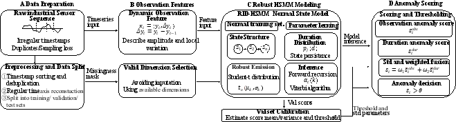
Figure 1 illustrates the overall framework. Raw sensor data are sorted by timestamp, deduplicated, aligned to a regular time axis, and divided into training, validation, and test sets. The model then constructs dynamic observation features, estimates a robust normal-state HSMM using only valid observation dimensions, performs forward inference and Viterbi decoding, and finally generates an anomaly score from the observation likelihood and duration deviation.

3.1. Observation Features and Valid-Dimension Student’s t Emissions

Industrial monitoring sequences often contain missing samples on a regular time grid. To prevent pseudo-observations from entering the probability model, RID-HSMM does not impose numerical imputation at missing positions. Instead, it constructs observation features and evaluates the state-conditioned density only over the valid dimensions.

Let the raw monitoring sequence on the regular time axis be:

y_{1 : T} = \{y_{1}, y_{2}, . . ., y_{T}\}

(8)

To capture both amplitude and local dynamics, the observation vector

x_{t}

at time

t

is defined as:

x_{t} = {(x_{t, 1}, x_{t, 2})}^{Τ} = {(y_{t}, Δ y_{t})}^{Τ}

(9)

Because either

y_{t}

y_{t - 1}

may be missing,

Δ y_{t}

is available only when both adjacent observations are available. Let

m \in \{1, 2\}

denote the feature index, where

m = 1

corresponds to the measured value and

m = 2

corresponds to the first-order difference.

Download: Download full-size image

Figure 1. Framework of RID-HSMM.

In state

k

, the Student’s t emission density for feature

m

f_{k, m} (x_{t, m}) = \frac{Γ (\frac{υ + 1}{2})}{Γ (\frac{υ}{2}) \sqrt{υπ} σ_{k, m}} {[1 + \frac{1}{υ} {(\frac{x_{t, m} - μ_{k, m}}{σ_{k, m}})}^{2}]}^{- \frac{υ + 1}{2}}

(10)

Here,

μ_{k, m}

and

σ_{k, m}

are the location and scale parameters of state

k

for feature

m

, and

υ

is the number of degrees of freedom. Student’s t emissions provide greater robustness than Gaussian emissions for monitoring data with spikes, drift, and heavy-tailed perturbations. Let

M_{t}

denote the set of feature dimensions that are available at time

t

. The emission density over valid dimensions is

{\tilde{b}}_{k} (x_{t}) = \prod_{m \in M_{t}} f_{k, m} (x_{t, m})

(11)

When both

y_{t}

and

y_{t - 1}

are available,

M_{t} = \{1, 2\}

and

{\tilde{b}}_{k} (x_{t}) = f_{k, 1} (y_{t}) f_{k, 2} (Δ y_{t})

(12)

When

y_{t}

is available but

Δ y_{t}

cannot be computed,

M_{t} = \{1\}

and

{\tilde{b}}_{k} (x_{t}) = f_{k, 1} (y_{t})

(13)

When

y_{t}

is missing, the time point contributes no observation-density term, and

{\tilde{b}}_{k} (x_{t})

is set to 1. In that case, state inference is driven by the transition probabilities and the duration distribution. The state-segment observation density in RID-HSMM is therefore

{\tilde{b}}_{k, d} (x_{[t + 1 : t + d]}) = \prod_{τ = t + 1}^{t + d} {\tilde{b}}_{k} (x_{τ})

(14)

Thus, RID-HSMM preserves the HSMM duration structure while preventing interpolated pseudo-observations from biasing the emission density. Student’s t emissions further improve robustness to local disturbances.

3.2. Forward Probability Recursion

Combining the HSMM recursion in Eq. (5) with the valid-dimension state-segment density in Eq. (14) yields the RID-HSMM forward recursion:

{\tilde{α}}_{u} (k) = \sum_{d = 1}^{\min (D, u)} \sum_{i \neq k}^{K} {\tilde{α}}_{u - d} (i) a_{ik} p_{k} (d) {\tilde{b}}_{k, d} (x_{[u - d + 1 : u]})

(15)

The marginal likelihood of the observed feature sequence is then

{\tilde{L}}_{u} = P (x_{[1 : u]}| λ) = \sum_{k = 1}^{K} {\tilde{α}}_{u} (k)

(16)

Eq. (16) quantifies how well the observed test sequence matches the normal-state RID-HSMM model.

3.3. Anomaly-Score Design

RID-HSMM is trained on normal operating data. During detection, a time point or state segment is considered suspicious if the current observation has a low probability under the normal model or if the decoded state duration deviates markedly from the learned normal duration distribution. The anomaly score therefore combines observation abnormality and duration abnormality.

From Eqs. (7) and (16), the observation anomaly score at time

t

is defined as the negative log predictive density:

s_{t}^{obs} = - Δ {\tilde{l}}_{u} = \log L_{u - 1} - \log L_{u}

(17)

This term measures the negative log predictive density of the current observation vector under the normal HSMM. To obtain a duration anomaly score, RID-HSMM uses Viterbi decoding to infer the most likely hidden state path. Consecutive samples with the same decoded state are merged into state segments. If a segment is assigned to state

k

and has duration

d

, the duration anomaly score for time points within the segment is

s_{t}^{dur} = - \frac{1}{d} \log p_{k} (d)

(18)

This term captures unusually short, unusually long, or otherwise atypical state-persistence patterns. Dividing by

d

converts the segment-level duration penalty into an average per-time-point score. Because

s_{t}^{obs}

and

s_{t}^{dur}

have different scales and meanings, both scores are standardized using the validation set. Let the standardized scores be

{\overset{̅}{s}}_{t}^{obs}

and

{\overset{̅}{s}}_{t}^{dur}

. The final anomaly score is

s_{t} = ω_{1} {\overset{̅}{s}}_{t}^{obs} + ω_{2} {\overset{̅}{s}}_{t}^{dur}

(19)

where

ω_{1}

and

ω_{2}

are the weights of the observation and duration components. The decision threshold

θ

is calibrated on the validation set. A time point is labeled as anomalous when

s_{t} > θ

In practice, the threshold can be adjusted according to operational risk tolerance. A higher upper-tail quantile or a larger standard-deviation multiplier produces a more conservative detector with fewer false alarms, whereas a lower threshold increases anomaly coverage and improves the detection rate at the cost of more false alarms. This calibration mechanism allows RID-HSMM to be adapted to different industrial alarm management requirements.

4. Experiments and Results

We evaluated the proposed method on a real monitoring sequence from a centrifugal compressor in an industrial compressor station. The compressor operates for long periods under fluctuating load, and its monitoring sequence exhibits operating-mode changes, strong temporal dependence, and nonstationarity. These characteristics make the data suitable for evaluating anomaly detection in industrial time series. All experiments were implemented in Python and executed on an Intel i5-12400F CPU / NVIDIA RTX 4060 GPU platform.

4.1. Dataset and Preprocessing

The motor-bearing temperature sequence was selected for univariate modeling. The sequence spans the period from 00:00:00 on 7 November 2022 to 00:00:00 on 29 November 2022. The nominal sampling interval inferred from the original timestamps was 1 min. Because field acquisition and storage included repeated reports, missing samples, and irregular timestamps, preprocessing consisted of timestamp sorting, duplicate timestamp removal, regular time-axis reconstruction, and marking original missing values.

After the regular time axis was reconstructed, the original sequence contained 31,680 time points and had a missing-data rate of 31.7%. After downsampling to 5 min, the sequence length was 6,336 and the missing data rate decreased to 2.7%. To evaluate anomaly detection under incomplete observations, the test set was further assessed under controlled missingness settings. These settings included the native missing positions in the 5-min sequence and additional missing samples or missing segments injected into the test set.

The downsampled incomplete sequence was split chronologically into training, validation, and test sets at a ratio of 60%, 20%, and 20%, respectively. The training set was used to learn an approximate normal operating pattern. The validation set was used to standardize anomaly indicators and determine the threshold. The test set was used to construct different missingness and anomaly injection scenarios. Synthetic anomaly labels in the test set were used only for evaluation and were not used in training or threshold selection.

4.2. Experimental Design, Baselines, and Evaluation Metrics

To evaluate performance under incomplete observations, we constructed 12 test scenarios by combining four missingness settings and three anomaly-rate settings. The missingness settings included the native missing positions in the downsampled 5-min sequence and additional missing rates of 10%, 20%, and 30%. The additional missingness was generated only in the test set and was not used for training or validation. The anomaly-rate settings were 5%, 10%, and 15%. Each missing-rate × anomaly-rate setting was repeated with four random seeds: 42, 35, 21, and 1. Precision (P), Detection Rate (DR), F1 score, and false-alarm rate (FAR) are computed as follows

[12]

P = \frac{TP}{TP + FP}

(20)

DR = \frac{TP}{TP + FN}

(21)

F 1 = \frac{2 TP}{2 TP + FP + FN}

(22)

FAR = \frac{FP}{FP + TN}

(23)

Here,

TP

is the number of correctly detected anomalous samples,

TN

is the number of correctly identified normal samples,

FP

is the number of normal samples incorrectly labeled as anomalous, and

FN

is the number of missed anomalous samples.

Missing observations and anomalous segments were injected into the test sequence. For each target missing rate, random missing samples and continuous missing segments were added to the existing missing positions to simulate random packet loss and continuous communication interruptions. Offset and drift anomalies were injected as continuous segments to represent common industrial phenomena such as measurement bias, slow degradation, and repeated readings. Let

τ

be the segment start time,

ι

be the segment length,

σ

be the standard deviation of the normal training sequence, and

μ

be the anomaly-strength coefficient. The injected offset and drift anomaly segments (

{\hat{y}}_{t}

and

{\tilde{y}}_{t}, respectively)

are defined as follows

[13]

{\hat{y}}_{t} = y_{t} + μσ

(24)

{\tilde{y}}_{t} = y_{t} + μσ \times \frac{t - τ}{ι - 1}

(25)

We compared RID-HSMM with ARIMA, robust median smoothing, Matrix Profile, LSTM-AE, and USAD. ARIMA represents a traditional prediction-residual baseline; robust median smoothing represents a local robust detector; Matrix Profile represents a distance-based subsequence-similarity detector; and LSTM-AE and USAD represent reconstruction-error deep-learning detectors. For baseline methods that cannot directly process missing values, linear interpolation was used to construct complete inputs under the same train/validation/test split, because it is deterministic, transparent, and introduces no additional model-specific hyperparameters. The imputation choice can influence prediction-error and reconstruction-error baselines because imputed values are used directly as model inputs. Smoother schemes, such as spline interpolation, may introduce additional assumptions about local curve smoothness, which can affect abrupt changes, offsets, and drift boundaries in industrial anomaly segments.

4.3. Anomaly Detection Performance

Table 1 reports the mean results of the six methods across the 12 missing-rate × anomaly-rate settings. Because this study focuses on continuous anomalous-segment detection in incomplete univariate industrial time series, we report point-level metrics, segment-level metrics, and the FAR. Point-level metrics quantify sample-wise classification; segment-level metrics evaluate whether anomaly events are captured continuously and stably, and FAR measures the proportion of normal samples incorrectly classified as anomalous.

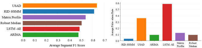
To better illustrate the trade-off between segment-level detection performance and false-alarm control, Figure 2 shows the segment-level F1 score and the average false-alarm rate reported in Table 1.

RID-HSMM achieved a segment-level F1 score of 0.613, which is slightly lower than the 0.638 obtained by USAD. The relative gap is approximately 3.9%, indicating that RID-HSMM approaches the segment-level detection performance of the strongest deep-learning baseline. Its main advantage lies in false-alarm control. RID-HSMM achieved the lowest average FAR of 0.030. Compared with USAD (0.362), the FAR was reduced by approximately 91.7%; compared with LSTM-AE (0.591), it was reduced by approximately 94.9%. RID-HSMM is therefore suitable for industrial alarm scenarios in which false alarms are costly and stable alarms are required.

Download: Download full-size image

Figure 2. Comparison of segment-level performance and false-alarm rate among different methods.

Table 1. Average performance of different methods across 12 missing-rate × anomaly-rate scenarios.

Method	Point-level			Segment-level			$FAR$
Method	$P$	$DR$	$F 1$	$P$	$DR$	$F 1$	$FAR$
RID-HSMM	0.544	0.321	0.396	0.762	0.527	0.613	0.030
USAD	0.223	0.877	0.348	0.621	0.715	0.638	0.362
Matrix Profile	0.275	0.442	0.329	0.486	0.653	0.539	0.124
Robust Median	0.392	0.548	0.451	0.407	0.701	0.505	0.092
LSTM-AE	0.168	0.971	0.282	0.770	0.409	0.487	0.591
ARIMA	0.297	0.373	0.325	0.344	0.821	0.478	0.093

At the point level, RID-HSMM achieved the highest precision (0.544), indicating that its predicted anomalous samples were more concentrated in true anomalous regions. Its point-level detection rate (0.321) was lower than those of USAD, LSTM-AE, and robust median smoothing, indicating a conservative decision strategy. This behavior is consistent with the low FAR: RID-HSMM suppresses scattered alarms through state-duration constraints and observation-density modeling.

The relatively low point-level detection rate should be considered together with the extremely low FAR. RID-HSMM uses a conservative threshold calibrated on validation scores and combines observation likelihood with state-duration deviation. This setting favors reliable alarms concentrated in high-confidence abnormal regions. In practical deployment, the threshold can be selected according to maintenance policy and risk tolerance. For safety-critical monitoring, a lower threshold can be used to increase DR and reduce missed anomalous samples. For routine condition monitoring, a higher threshold can be used to suppress false alarms and reduce unnecessary inspections. The reported default setting reflects a false-alarm-control configuration, which is important for industrial systems where frequent false alarms can lead to alarm fatigue and unnecessary maintenance actions.

USAD achieved the highest segment-level F1 score but had a much higher FAR, suggesting that part of its segment-detection ability resulted from wider alarm coverage. LSTM-AE reached the highest point-level detection rate but also the highest FAR, indicating that reconstruction models are sensitive to imputation errors and local fluctuations in incomplete univariate sequences. ARIMA and robust median smoothing achieved relatively high detection rates in some settings but had lower segment-level precision and F1 scores, reflecting fragmented alarms. Matrix Profile maintained a relatively low FAR but still underperformed RID-HSMM in segment-level F1, suggesting that subsequence similarity alone is insufficient to model state-duration structure under missing observations.

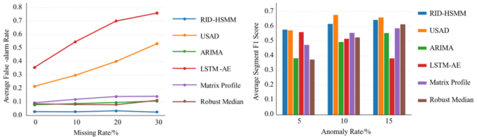
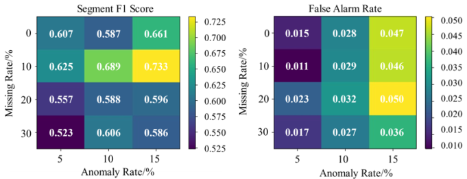
To further assess how the detection performance changes with missingness and anomaly prevalence, Figure 3 shows the trends in the average false-alarm rate and segment-level F1 score for all methods under different scenario settings Figure 4 further summarizes the distribution of the segment-level F1 score and false-alarm rate achieved by RID-HSMM across the 12 combinations of missing rate and anomaly rate.

Download: Download full-size image

Figure 3. Sensitivity of detection performance to missingness and anomaly prevalence.

Download: Download full-size image

Figure 4. Performance of RID-HSMM across the 12 missing-rate × anomaly-rate scenarios.

Across the 0–30% missing-rate settings, RID-HSMM maintained a low FAR because unavailable positions do not enter the emission-density calculation as interpolated values. When only part of the observation vector is available, the likelihood is evaluated on the valid dimensions; when the measured value is unavailable, the time point contributes no observation density and inference relies on transition and duration information. This mechanism reduces the propagation of interpolation errors into anomaly scores and explains the stable false-alarm control under increasing missingness. This behavior is consistent with the RID-HSMM design: missing positions are not forcibly imputed, and only actually observed feature dimensions contribute to the emission density. In contrast, deep reconstruction models require complete inputs; as the missing rate increases, interpolation error enters the reconstruction error and spreads the anomaly-score distribution, thereby increasing false alarms.

As the anomaly rate increased, the segment-level F1 score of RID-HSMM increased slightly because stronger segment evidence makes observation-density and duration deviations easier to combine into continuous decision signals. The FAR remained low, showing that the model maintained false-alarm control while detection evidence increased.

4.4. Component Analysis of RID-HSMM

To evaluate the contribution of each design component in RID-HSMM, we conducted component-level comparisons at a 10% missing rate and a 10% anomaly rate, in which selected mechanisms were removed or replaced by conventional alternatives. The full RID-HSMM uses emission density over valid dimensions, Student’s t emissions, first-order difference features, and duration anomaly scoring.

Replacing Student’s t emissions with Gaussian emissions reduced point-level precision from 0.591 to 0.311 and segment-level precision from 0.831 to 0.540. This result indicates that Student’s t emissions improve robustness to heavy-tailed disturbances and outliers in sequences containing spikes, offsets, and local perturbations.

Removing the duration anomaly score reduced segment-level detection rate from 0.831 to 0.455 and segment-level F1 from 0.689 to 0.498. Observation abnormality alone was insufficient for stable continuous-segment detection. The duration-deviation term adds sequential-structure constraints, suppresses fragmented alarms, and improves segment-level recognition. Removing the first-order difference feature reduced segment-level detection rate to 0.281 and segment-level F1 to 0.346, demonstrating that amplitude-only modeling was not sensitive enough to local changes, slow drift, and segment boundaries. Finally, the conventional HSMM had substantially lower segment-level precision and F1 than the complete RID-HSMM. The performance gain therefore arises from the combined effects of valid-dimension emission-density evaluation, Student’s t robustness, dynamic difference features, and duration-based anomaly scoring.

Table 2. Component-level comparison results of RID-HSMM.

	Point-level			Segment-level
	$P$	$DR$	$F 1$	$P$	$DR$	$F 1$
Full	0.591	0.354	0.438	0.831	0.621	0.689
w/o Student’s t emissions	0.311	0.617	0.410	0.540	0.859	0.661
w/o duration score	0.326	0.407	0.353	0.455	0.613	0.498
w/o first-order difference	0.425	0.217	0.279	0.508	0.281	0.346
HSMM	0.424	0.266	0.322	0.275	0.585	0.373

Note: “Full” refers to the complete RID-HSMM configuration. “w/o” denotes “without”, meaning that a specific component is removed or replaced by a standard alternative. In “w/o Student’s t emissions”, the Student’s t emission distribution is replaced by a Gaussian emission distribution. In “w/o duration score”, the state-duration anomaly term is excluded from the anomaly score, leaving only the observation-based anomaly term in the score. In “w/o first-order difference”, the feature vector is reduced to the raw observed value only. “HSMM” denotes the conventional HSMM applied after linear interpolation of missing values.

4.5. Preliminary External Validation

To examine whether RID-HSMM depends on a particular station, unit, or sensor variable, we further evaluated the method on data from different stations, compressor units, and sensor variables. The results are summarized in Table 3.

RID-HSMM achieved the highest average segment-level F1 score (0.521). Compared with LSTM-AE, USAD, ARIMA, robust median smoothing, and Matrix Profile, the segment-level F1 score was higher by approximately 8.7%, 11.2%, 12.5%, 23.4%, and 59.2%, respectively. These results indicate that RID-HSMM could still identify sustained anomalous segments when the station, unit, and sensor variable change; its performance is not limited to the main experimental dataset.

Table 3. External validation results.

Method	Point-level F1	Segment-level F1	FAR
RID-HSMM	0.312	0.521	0.026
LSTM-AE	0.245	0.479	0.172
USAD	0.203	0.468	0.756
ARIMA	0.376	0.463	0.167
Robust Median	0.359	0.422	0.021
Matrix Profile	0.148	0.327	0.112

RID-HSMM obtained an average FAR of 0.026. Although this value is slightly higher than that of robust median smoothing (0.021), it is substantially lower than those of LSTM-AE (0.172), ARIMA (0.167), and USAD (0.756). Compared with USAD and LSTM-AE, RID-HSMM reduced FAR by approximately 96.6% and 85.1%, respectively. These results suggest that deep reconstruction models are vulnerable to imputation error and local fluctuations in incomplete univariate sequences, whereas RID-HSMM achieved a more stable balance between segment-level detection and false-alarm suppression through missing-data handling without numerical imputation, Student’s t emissions, and explicit duration constraints. Robust median smoothing produced the lowest FAR but had a lower segment-level F1 score than RID-HSMM, indicating that local statistical methods can suppress false alarms but have limited ability to identify sustained anomaly segments.

5. Conclusion

This study presents RID-HSMM, a robust hidden semi-Markov model for detecting sustained anomalous segments in incomplete centrifugal-compressor monitoring sequences. The method constructs a two-dimensional feature from the measured value and its adjacent first-order difference, evaluates emission likelihoods only over available feature dimensions, introduces Student’s t emissions to improve robustness to heavy-tailed disturbances, and combines negative log predictive density with state-duration deviation for anomaly scoring.

Experiments on real compressor monitoring data showed that RID-HSMM achieved the highest point-level precision and the lowest false-alarm rate, while its segment-level F1 score was close to that of the strongest deep reconstruction baseline. Component-removal and replacement analyses indicated that the main design components contribute jointly to false-alarm suppression and segment-level anomaly detection.

External validation provides preliminary evidence that RID-HSMM could maintain stable performance across different compressor units and monitoring variables. The results indicate that explicitly modeling state duration and avoiding pseudo-observations are effective strategies for anomaly detection in incomplete industrial time series.

Abbreviations

HMM	Hidden Markov Model
HSMM	Hidden Semi-Markov Model
RID-HSMM	Robust Incomplete-Data Hidden Semi-Markov Model
ARIMA	Autoregressive Integrated Moving Average
LSTM-AE	Long Short-Term Memory Autoencoder
USAD	Unsupervised Anomaly Detection
P	Precision
DR	Detection Rate
FAR	False-Alarm Rate

Author Contributions

Rongsong Zhang: Conceptualization, Formal Analysis, Investigation, Methodology, Software, Visualization, Writing – original draft

Enyun Liang: Data curation, Validation

Shaolin Hu: Funding acquisition, Project administration, Resources, Supervision

Ye Ke: Writing – review & editing

Funding

This work is supported by the National Natural Science Foundation of China (62373115) and the Natural Science Foundation of Guangdong Province (2024A1515010870).

Conflicts of Interest

The authors declare no conflicts of interest.

References

[1]	Wang, Y., Hu, S. State monitoring and fault prediction of centrifugal compressors based on long short-term memory and principal component analysis (LSTM-PCA). PeerJ Computer Science. 2024, 10, e2433. https://doi.org/10.7717/peerj-cs.2433
[2]	Xiao, F., Fan, J. Unsupervised anomaly detection in the presence of missing values. In Advances in Neural Information Processing Systems 37 (NeurIPS 2024), Vancouver, Canada, 2024; pp. 138130-138162.
[3]	Toller, M. B., Geiger, B. C., Kern, R. Detecting abrupt changes in missing time series data. Information Sciences. 2025, 717, 122322. https://doi.org/10.1016/j.ins.2025.122322
[4]	Lu, Y., Wu, R., Mueen, A., Zuluaga, M. A., Keogh, E. Matrix Profile XXIV: scaling time series anomaly detection to trillions of datapoints and ultra-fast arriving data streams. In Proceedings of the 28th ACM SIGKDD Conference on Knowledge Discovery and Data Mining, Washington, DC, USA, 2022; pp. 1173-1182. https://doi.org/10.1145/3534678.3539271
[5]	Tan, X., Xi, H. Hidden semi-Markov model for anomaly detection. Applied Mathematics and Computation. 2008, 205(2), 562-567. https://doi.org/10.1016/j.amc.2008.05.028
[6]	Zhao, H., Wang, Y., Sun, A. A water intake anomaly detection method based on ARIMA model and 3σ criterion. Water Resources Informatization. 2022, (1), 35-41. https://doi.org/10.19364/j.1674-9405.2022.01.008
[7]	Chen, L., Qin, K., Hao, K. Time series anomaly detection method based on integrated LSTM-AE. Journal of Huazhong University of Science and Technology (Natural Science Edition). 2021, 49(11), 35-40. https://doi.org/10.13245/j.hust.211107
[8]	Audibert, J., Michiardi, P., Guyard, F., Marti, S., Zuluaga, M. A. USAD: Unsupervised anomaly detection on multivariate time series. In Proceedings of the 26th ACM SIGKDD International Conference on Knowledge Discovery & Data Mining, Virtual Event, CA, USA, 2020; pp. 3395-3404. https://doi.org/10.1145/3394486.3403392
[9]	Yu, S. Z., Kobayashi, H. A hidden semi-Markov model with missing data and multiple observation sequences for mobility tracking. Signal Processing. 2003, 83(2), 235-250. https://doi.org/10.1016/S0165-1684(02)00378-X
[10]	Yu, S. Z. Hidden semi-Markov models. Artificial Intelligence. 2010, 174(2), 215-243. https://doi.org/10.1016/j.artint.2009.11.011
[11]	Ding, J., Shah, S. A robust hidden semi-Markov model with application to aCGH data processing. International Journal of Data Mining and Bioinformatics. 2013, 8(4), 427-442. https://doi.org/10.1504/IJDMB.2013.056616
[12]	Chen, Z., Li, Z., Huang, J., Liu, S., Long, H. An effective method for anomaly detection in industrial Internet of Things using XGBoost and LSTM. Scientific Reports. 2024, 14, 23969. https://doi.org/10.1038/s41598-024-74822-6
[13]	Jia, L., Cornelis, B., Gryllias, K. Validation of time series anomaly detection methods for automated detection of measurement anomalies in noise and vibration testing. In Proceedings of ISMA 2024 - International Conference on Noise and Vibration Engineering and USD 2024, Leuven, Belgium, 2024.

Cite This Article

Plain Text BibTeX RIS

APA Style

Zhang, R., Liang, E., Hu, S., Ke, Y. (2026). A Robust Hidden Semi-Markov Model for Anomaly Detection of Centrifugal Compressors Monitoring Data with Missing Values. International Journal on Data Science and Technology, 12(2), 24-34. https://doi.org/10.11648/j.ijdst.20261202.11

Copy | Download

ACS Style

Zhang, R.; Liang, E.; Hu, S.; Ke, Y. A Robust Hidden Semi-Markov Model for Anomaly Detection of Centrifugal Compressors Monitoring Data with Missing Values. Int. J. Data Sci. Technol. 2026, 12(2), 24-34. doi: 10.11648/j.ijdst.20261202.11

Copy | Download

AMA Style

Zhang R, Liang E, Hu S, Ke Y. A Robust Hidden Semi-Markov Model for Anomaly Detection of Centrifugal Compressors Monitoring Data with Missing Values. Int J Data Sci Technol. 2026;12(2):24-34. doi: 10.11648/j.ijdst.20261202.11

Copy | Download

@article{10.11648/j.ijdst.20261202.11,
  author = {Rongsong Zhang and Enyun Liang and Shaolin Hu and Ye Ke},
  title = {A Robust Hidden Semi-Markov Model for Anomaly Detection of Centrifugal Compressors Monitoring Data with Missing Values},
  journal = {International Journal on Data Science and Technology},
  volume = {12},
  number = {2},
  pages = {24-34},
  doi = {10.11648/j.ijdst.20261202.11},
  url = {https://doi.org/10.11648/j.ijdst.20261202.11},
  eprint = {https://article.sciencepublishinggroup.com/pdf/10.11648.j.ijdst.20261202.11},
  abstract = {Centrifugal compressors are critical rotating machines in petrochemical and energy systems, and abnormal operating states may lead to unplanned shutdowns, efficiency loss, and safety risks. In practical monitoring systems, sensor data often contain missing samples, local disturbances, and sustained anomalous segments, making conventional pointwise and interpolation-dependent anomaly detectors less reliable. To address these issues, this paper presents a robust incomplete-data hidden semi-Markov model (RID-HSMM) for anomaly detection in monitoring data from centrifugal compressors. The method constructs a two-dimensional observation vector from each observed value and its adjacent first-order difference to represent both amplitude information and local dynamic variation. To avoid treating interpolated values as real observations, the emission likelihood is only evaluated over the available observed feature dimensions. A Student’s t distribution is used as the emission model to improve robustness against heavy-tailed disturbances and local outliers. In the anomaly detection phase, the anomaly score combines the negative log predictive density of the observations and the state-duration deviation, thereby capturing both observation abnormality and state-persistence abnormality. Experiments on real motor-bearing temperature data from a centrifugal compressor were conducted under multiple missingness and anomaly settings. Compared with ARIMA, Matrix Profile, LSTM-AE, USAD, and the robust median baselines, RID-HSMM achieved the highest point-level precision and the lowest false-alarm rate, while maintaining competitive segment-level detection performance. The results indicate that explicit state-duration modeling and pseudo-observation avoidance can improve the reliability of anomaly detection for incomplete industrial time series.},
 year = {2026}
}

Copy | Download

TY  - JOUR
T1  - A Robust Hidden Semi-Markov Model for Anomaly Detection of Centrifugal Compressors Monitoring Data with Missing Values
AU  - Rongsong Zhang
AU  - Enyun Liang
AU  - Shaolin Hu
AU  - Ye Ke
Y1  - 2026/07/24
PY  - 2026
N1  - https://doi.org/10.11648/j.ijdst.20261202.11
DO  - 10.11648/j.ijdst.20261202.11
T2  - International Journal on Data Science and Technology
JF  - International Journal on Data Science and Technology
JO  - International Journal on Data Science and Technology
SP  - 24
EP  - 34
PB  - Science Publishing Group
SN  - 2472-2235
UR  - https://doi.org/10.11648/j.ijdst.20261202.11
AB  - Centrifugal compressors are critical rotating machines in petrochemical and energy systems, and abnormal operating states may lead to unplanned shutdowns, efficiency loss, and safety risks. In practical monitoring systems, sensor data often contain missing samples, local disturbances, and sustained anomalous segments, making conventional pointwise and interpolation-dependent anomaly detectors less reliable. To address these issues, this paper presents a robust incomplete-data hidden semi-Markov model (RID-HSMM) for anomaly detection in monitoring data from centrifugal compressors. The method constructs a two-dimensional observation vector from each observed value and its adjacent first-order difference to represent both amplitude information and local dynamic variation. To avoid treating interpolated values as real observations, the emission likelihood is only evaluated over the available observed feature dimensions. A Student’s t distribution is used as the emission model to improve robustness against heavy-tailed disturbances and local outliers. In the anomaly detection phase, the anomaly score combines the negative log predictive density of the observations and the state-duration deviation, thereby capturing both observation abnormality and state-persistence abnormality. Experiments on real motor-bearing temperature data from a centrifugal compressor were conducted under multiple missingness and anomaly settings. Compared with ARIMA, Matrix Profile, LSTM-AE, USAD, and the robust median baselines, RID-HSMM achieved the highest point-level precision and the lowest false-alarm rate, while maintaining competitive segment-level detection performance. The results indicate that explicit state-duration modeling and pseudo-observation avoidance can improve the reliability of anomaly detection for incomplete industrial time series.
VL  - 12
IS  - 2
ER  -

Copy | Download

Author Information

Rongsong Zhang

School of Automation, Guangdong University of Petrochemical Technology, Maoming, China

Biography: Rongsong Zhang is a postgraduate student majoring in Control Engineering at the School of Automation, Guangdong University of Petrochemical Technology, and is one of Prof. Shaolin Hu’s students. His research area is diagnosis of industrial instrumentation data.

http://orcid.org/0009-0003-9726-9830
Enyun Liang

School of Automation, Guangdong University of Petrochemical Technology, Maoming, China

Biography: Enyun Liang is a laboratory technician in the School of Automation, Guangdong University of Petrochemical Technology. She received her Bachelor’s degree from Guangdong University of Petrochemical Technology in 2019, Master’s degree from Guangdong University of Technology in 2022. Her research area focuses on equipment fault diagnosis and digital twins.
Shaolin Hu

School of Automation, Guangdong University of Petrochemical Technology, Maoming, China

Biography: Rongsong Zhang is a postgraduate student majoring in Control Engineering at the School of Automation, Guangdong University of Petrochemical Technology, and is one of Prof. Shaolin Hu’s students. His research area is diagnosis of industrial instrumentation data.

Contact Email

http://orcid.org/0000-0001-7589-8474
Ye Ke

School of Automation, Guangdong University of Petrochemical Technology, Maoming, China

Biography: Ye Ke a research assistant in the School of Automation, Guangdong University of Petrochemical Technology. He received his Bachelor’s degree from University of Macau in 2018, Master’s degree from Nanyang Technological University in 2019. His research area focuses on automation instrumentation, process monitoring and control, system safety.

http://orcid.org/0000-0001-6467-3448

Download PDF

Submit an Article

Plain Text BibTeX RIS

APA Style

Zhang, R., Liang, E., Hu, S., Ke, Y. (2026). A Robust Hidden Semi-Markov Model for Anomaly Detection of Centrifugal Compressors Monitoring Data with Missing Values. International Journal on Data Science and Technology, 12(2), 24-34. https://doi.org/10.11648/j.ijdst.20261202.11

Copy | Download

ACS Style

Zhang, R.; Liang, E.; Hu, S.; Ke, Y. A Robust Hidden Semi-Markov Model for Anomaly Detection of Centrifugal Compressors Monitoring Data with Missing Values. Int. J. Data Sci. Technol. 2026, 12(2), 24-34. doi: 10.11648/j.ijdst.20261202.11

Copy | Download

AMA Style

Zhang R, Liang E, Hu S, Ke Y. A Robust Hidden Semi-Markov Model for Anomaly Detection of Centrifugal Compressors Monitoring Data with Missing Values. Int J Data Sci Technol. 2026;12(2):24-34. doi: 10.11648/j.ijdst.20261202.11

Copy | Download

@article{10.11648/j.ijdst.20261202.11,
  author = {Rongsong Zhang and Enyun Liang and Shaolin Hu and Ye Ke},
  title = {A Robust Hidden Semi-Markov Model for Anomaly Detection of Centrifugal Compressors Monitoring Data with Missing Values},
  journal = {International Journal on Data Science and Technology},
  volume = {12},
  number = {2},
  pages = {24-34},
  doi = {10.11648/j.ijdst.20261202.11},
  url = {https://doi.org/10.11648/j.ijdst.20261202.11},
  eprint = {https://article.sciencepublishinggroup.com/pdf/10.11648.j.ijdst.20261202.11},
  abstract = {Centrifugal compressors are critical rotating machines in petrochemical and energy systems, and abnormal operating states may lead to unplanned shutdowns, efficiency loss, and safety risks. In practical monitoring systems, sensor data often contain missing samples, local disturbances, and sustained anomalous segments, making conventional pointwise and interpolation-dependent anomaly detectors less reliable. To address these issues, this paper presents a robust incomplete-data hidden semi-Markov model (RID-HSMM) for anomaly detection in monitoring data from centrifugal compressors. The method constructs a two-dimensional observation vector from each observed value and its adjacent first-order difference to represent both amplitude information and local dynamic variation. To avoid treating interpolated values as real observations, the emission likelihood is only evaluated over the available observed feature dimensions. A Student’s t distribution is used as the emission model to improve robustness against heavy-tailed disturbances and local outliers. In the anomaly detection phase, the anomaly score combines the negative log predictive density of the observations and the state-duration deviation, thereby capturing both observation abnormality and state-persistence abnormality. Experiments on real motor-bearing temperature data from a centrifugal compressor were conducted under multiple missingness and anomaly settings. Compared with ARIMA, Matrix Profile, LSTM-AE, USAD, and the robust median baselines, RID-HSMM achieved the highest point-level precision and the lowest false-alarm rate, while maintaining competitive segment-level detection performance. The results indicate that explicit state-duration modeling and pseudo-observation avoidance can improve the reliability of anomaly detection for incomplete industrial time series.},
 year = {2026}
}

Copy | Download

TY  - JOUR
T1  - A Robust Hidden Semi-Markov Model for Anomaly Detection of Centrifugal Compressors Monitoring Data with Missing Values
AU  - Rongsong Zhang
AU  - Enyun Liang
AU  - Shaolin Hu
AU  - Ye Ke
Y1  - 2026/07/24
PY  - 2026
N1  - https://doi.org/10.11648/j.ijdst.20261202.11
DO  - 10.11648/j.ijdst.20261202.11
T2  - International Journal on Data Science and Technology
JF  - International Journal on Data Science and Technology
JO  - International Journal on Data Science and Technology
SP  - 24
EP  - 34
PB  - Science Publishing Group
SN  - 2472-2235
UR  - https://doi.org/10.11648/j.ijdst.20261202.11
AB  - Centrifugal compressors are critical rotating machines in petrochemical and energy systems, and abnormal operating states may lead to unplanned shutdowns, efficiency loss, and safety risks. In practical monitoring systems, sensor data often contain missing samples, local disturbances, and sustained anomalous segments, making conventional pointwise and interpolation-dependent anomaly detectors less reliable. To address these issues, this paper presents a robust incomplete-data hidden semi-Markov model (RID-HSMM) for anomaly detection in monitoring data from centrifugal compressors. The method constructs a two-dimensional observation vector from each observed value and its adjacent first-order difference to represent both amplitude information and local dynamic variation. To avoid treating interpolated values as real observations, the emission likelihood is only evaluated over the available observed feature dimensions. A Student’s t distribution is used as the emission model to improve robustness against heavy-tailed disturbances and local outliers. In the anomaly detection phase, the anomaly score combines the negative log predictive density of the observations and the state-duration deviation, thereby capturing both observation abnormality and state-persistence abnormality. Experiments on real motor-bearing temperature data from a centrifugal compressor were conducted under multiple missingness and anomaly settings. Compared with ARIMA, Matrix Profile, LSTM-AE, USAD, and the robust median baselines, RID-HSMM achieved the highest point-level precision and the lowest false-alarm rate, while maintaining competitive segment-level detection performance. The results indicate that explicit state-duration modeling and pseudo-observation avoidance can improve the reliability of anomaly detection for incomplete industrial time series.
VL  - 12
IS  - 2
ER  -

Copy | Download