Abstract
Selecting an appropriate deep learning architecture for pipeline Remaining Useful Life (RUL) prediction requires a systematic comparison under consistent experimental conditions. This revision reports results computed directly on the dataset (500 records spanning 12 installation cohorts from 2000–2024; see Section 3.1). We benchmark Long Short-Term Memory (LSTM) networks, Convolutional Neural Networks (CNN), and Graph Neural Networks (GNN) against a common Artificial Neural Network (ANN) baseline using identical preprocessing and seven-fold stratified cross-validation (Section 3.1 explains why the originally proposed expanding-window temporal cross-validation could not be applied to the data received). The ANN, LSTM, and GNN are statistically distinguishable but practically tied at near-perfect regression performance (GNN: R2 = 0.9998; ANN: R2 = 0.9996; LSTM: R2 = 0.9986; all p < 0.05 pairwise, Section 7.4) and all three achieve perfect binary classification (Accuracy = Precision = Recall = F1 = 1.000). The CNN performs far worse on both tasks (R2 = 0.1655; classification F1 = 0.373), which we attribute to its translation-invariant, weight-shared convolutional structure being poorly suited to a tabular prediction task in which each input feature requires its own, non-interchangeable coefficient (Section 8.2). Direct analysis of the target variable shows that Remaining Useful Life is an exact deterministic linear function of five input covariates (R2 = 1.0000 for ordinary linear regression; Section 3.1.1), which explains why every architecture capable of learning feature-specific weights (ANN, LSTM, GNN) recovers it almost perfectly, and an ablation test shows the GNN’s graph-convolution step contributes negligibly (R2 changes from 0.9998 to 0.9995 when message-passing is disabled), providing no support for the originally hypothesised spatial-relationship-modelling advantage. These findings substantially revise the architecture-selection guidance proposed in the original submission: rather than recommending the GNN as the default architecture, we recommend the ANN as the default choice on the grounds of statistically indistinguishable accuracy at a fraction of the computational cost (Section 3.5), and we recommend against the standard (translation-invariant) CNN for tabular pipeline-attribute prediction tasks of this kind.
|
Published in
|
Science Discovery Artificial Intelligence (Volume 1, Issue 4)
|
|
DOI
|
10.11648/j.sdai.20260104.12
|
|
Page(s)
|
147-159 |
|
Creative Commons
|

This is an Open Access article, distributed under the terms of the Creative Commons Attribution 4.0 International License (http://creativecommons.org/licenses/by/4.0/), which permits unrestricted use, distribution and reproduction in any medium or format, provided the original work is properly cited.
|
|
Copyright
|
Copyright © The Author(s), 2026. Published by Science Publishing Group
|
Keywords
Deep Learning, LSTM, CNN, GNN, ANN, Pipeline Degradation, Remaining Useful Life, Nigeria
1. Introduction
The integrity of oil and gas pipelines is a matter of critical national importance, particularly in Nigeria, where pipeline failures contribute to environmental damage, economic losses, and safety hazards across the Niger Delta and beyond
| [4] | Eze, C. C., Okafor, J. I., and Nwankwo, T. C. (2023). Geospatial analysis of pipeline failure clustering in Nigeria. International Journal of Environmental Studies, 80(7), 1204–1219. |
[4]
. Accurate prediction of Remaining Useful Life (RUL) enables operators to prioritise maintenance, reduce unplanned shutdowns, and optimise inspection schedules. Over the past decade, deep learning techniques have emerged as powerful tools for this purpose. Yet, the proliferation of individual architecture studies — each reporting strong results on different datasets under different experimental conditions — has made it difficult for practitioners to select the most appropriate method for a given operational context.
LSTM networks have been widely advocated for their temporal sequence modelling capacity
| [6] | Gholami, H., Anbarjafari, G., and Roshanaei, H. (2021). Long short-term memory networks for remaining useful life prediction in pipeline systems. IEEE Access, 6, 38447–38458. |
| [13] | Shaik, N. B., Pedapati, S. R., Taqvi, S. A. A., Othman, A. R., and Dzubir, F. A. A. (2022). Recurrent neural network-based model for estimating the life condition of a dry gas pipeline. Process Safety and Environmental Protection, 164, 639–650. |
| [18] | Zhang, Z., and Li, H. (2021). Reliability analysis using the exponentiated Weibull distribution for pipeline lifespan estimation. Applied Mathematical Modelling, 85, 275–287. |
[6, 13, 18]
; CNN architectures for their spatial pattern extraction capability
| [5] | Farahat, A., Effenberger, F., and Vinck, M. (2023). A novel feature-scrambling approach reveals the capacity of convolutional neural networks to learn spatial relations. Neural Networks, 167, 400–414.
https://doi.org/10.1016/j.neunet.2023.08.021 |
| [15] | Sharma, R., and Gupta, M. (2022). Convolutional neural networks for pipeline condition monitoring. International Journal of Industrial Automation and Control, 15(3), 165–173. |
[5, 15]
; and GNNs for their ability to represent inter-segment dependencies in pipeline networks
| [3] | Chen, X., and Zhao, W. (2021). Graph neural networks for pipeline segment interdependency modelling. IEEE Transactions on Neural Networks and Learning Systems, 32(7), 3012–3021. |
| [7] | Huang, Z., He, Y., and Sick, B. (2023). Spatio-temporal attention graph neural network for remaining useful life prediction. Proceedings of the International Conference on Computational Science and Computational Intelligence (CSCI'23), IEEE. (Accepted, peer-reviewed conference paper; originally circulated as arXiv:2401.15964 — authors should confirm final proceedings page numbers before publication.) |
| [9] | Liu, M., Thompson, N., and Andersson, P. (2024). Graph neural networks for spatial failure propagation modelling in pipelines. Neural Networks, 157, 105–121. |
[3, 7, 9]
. However, because these studies use different datasets, preprocessing pipelines, cross-validation strategies, and performance metrics, their findings cannot be meaningfully compared. A practitioner seeking to select the most appropriate architecture for a Nigerian pipeline prediction task has no principled basis for choice beyond the architecture’s theoretical inductive bias.
This study addresses this gap through a controlled, systematic comparison. All four architectures — ANN, LSTM, CNN, and GNN — are applied to the same Nigerian pipeline dataset with identical preprocessing, the same expanding-window temporal cross-validation protocol, and the same suite of regression (R2, RMSE, MAE) and classification (Accuracy, Precision, Recall, F1-Score) metrics (RMSE: Root Mean Square Error; MAE: Mean Absolute Error). The comparison is not designed to declare a single winner, but rather to characterise the strengths and limitations of each architecture within the specific operational context of Nigerian pipeline degradation prediction, providing the empirical foundation needed to justify a hybrid ensemble integration that combines all four architectures.
1.1. Research Questions
This paper addresses three research questions:
1) Which deep learning architecture achieves the strongest regression performance for continuous RUL prediction on Nigerian pipeline data, and by what margin?
2) Does the same architecture also achieve the strongest classification performance for binary failure prediction, or do regression and classification tasks favour different architectures?
3) Are the performance differences between architectures attributable to their theoretical inductive biases, and do the results confirm the complementarity required for an effective hybrid ensemble?
1.2. Statement of the Problem
Pipeline degradation in Nigeria’s oil and gas sector is driven by complex interactions among environmental, operational, and structural factors, including corrosion, pressure fluctuations, soil conductivity, and ageing infrastructure. Traditional inspection and maintenance schedules are largely reactive, responding to failures rather than anticipating them. Whilst deep learning methods have demonstrated promise in predicting RUL and binary failure risk, no study has yet compared ANNs, LSTMs, CNNs, and GNNs under identical conditions on Nigerian pipeline data. The absence of such a controlled benchmark leaves practitioners without evidence-based guidance for architecture selection in this operationally critical context.
1.3. Aims and Objectives
The primary aim of this study is to provide a rigorous, controlled benchmark comparison of four deep learning architectures — ANN, LSTM, CNN, and GNN — for pipeline RUL prediction using Nigerian oil and gas data, in order to generate architecture-selection guidance grounded in empirical evidence.
The specific objectives are:
1) To apply all four architectures to a shared Nigerian pipeline dataset under identical preprocessing and evaluation conditions.
2) To evaluate regression performance using R2, RMSE, and MAE, and classification performance using Accuracy, Precision, Recall, and F1-Score.
3) To assess whether observed performance differences are consistent with each architecture’s theoretical inductive bias.
4) To confirm the complementarity of the four architectures as a justification for hybrid ensemble integration.
2. Literature Review
2.1. Artificial Neural Networks in Pipeline Integrity
Feedforward ANN models have long served as the baseline method for pipeline failure prediction. Their capacity as universal function approximators, formally established by Barron
| [1] | Barron, A. R. (1993). Universal approximation bounds for superpositions of a sigmoidal function. IEEE Transactions on Information Theory, 39(3), 930–945. |
[1]
, makes them applicable to a wide range of regression and classification tasks without imposing structural assumptions on the data. In the context of pipeline management, ANNs have been used to estimate corrosion rates, predict pressure drops, and classify failure risk from static feature vectors. Their computational efficiency and interpretability make them well-suited as non-redundant baselines against which more specialised architectures can be benchmarked.
2.2. LSTM Networks for Temporal Degradation Modelling
LSTM networks were specifically designed to overcome the vanishing gradient problem in recurrent neural networks, enabling the capture of long-range temporal dependencies
| [2] | Chen, L., and Zhang, Q. (2022). Long short-term memory networks for sequence modelling in predictive maintenance. Journal of Machine Learning Applications, 11(2), 112–128. |
[2]
. Zhang and Li
| [18] | Zhang, Z., and Li, H. (2021). Reliability analysis using the exponentiated Weibull distribution for pipeline lifespan estimation. Applied Mathematical Modelling, 85, 275–287. |
[18]
demonstrated their effectiveness for pipeline corrosion prediction using historical sensor sequences, whilst Shaik
et al | [13] | Shaik, N. B., Pedapati, S. R., Taqvi, S. A. A., Othman, A. R., and Dzubir, F. A. A. (2022). Recurrent neural network-based model for estimating the life condition of a dry gas pipeline. Process Safety and Environmental Protection, 164, 639–650. |
[13]
applied LSTM to estimate the life condition of dry gas pipelines, consistently outperforming ARIMA (AutoRegressive Integrated Moving Average) and classical time-series approaches. Gholami
et al | [6] | Gholami, H., Anbarjafari, G., and Roshanaei, H. (2021). Long short-term memory networks for remaining useful life prediction in pipeline systems. IEEE Access, 6, 38447–38458. |
[6]
further validated LSTM for RUL prediction from sequential degradation data. Ma
et al | [10] | Ma, Y., Shang, Z., Zheng, J., Zhang, Y., Weng, G., Zhao, S., and Bi, C. (2025). Research on leak detection and localisation for oil and gas pipelines using wavelet denoising with LSTM transformer models. Sensors, 25(8), 2411. |
[10]
extended LSTM to pipeline leak detection and localisation by combining it with wavelet denoising, demonstrating flexibility beyond pure regression. These studies consistently highlight LSTM’s advantage in capturing slow degradation trends spanning months or years, whilst also indicating that its performance degrades when the dominant predictive signal is cross-sectional rather than temporal.
2.3. Convolutional Neural Networks for Spatial Feature Extraction
CNNs have been shown to operate as learnable spatial smoothers that converge optimally with respect to the spatial regularity of the underlying function
| [12] | Rodriguez, C., and Martinez, M. (2023). Statistical foundations of convolutional neural networks. Journal of Spatial Statistics, 10, 100180. |
[12]
. In pipeline monitoring contexts, Sharma and Gupta
| [15] | Sharma, R., and Gupta, M. (2022). Convolutional neural networks for pipeline condition monitoring. International Journal of Industrial Automation and Control, 15(3), 165–173. |
[15]
demonstrated that CNNs effectively capture spatial degradation patterns across multi-sensor arrays, whilst Farahat
et al | [5] | Farahat, A., Effenberger, F., and Vinck, M. (2023). A novel feature-scrambling approach reveals the capacity of convolutional neural networks to learn spatial relations. Neural Networks, 167, 400–414.
https://doi.org/10.1016/j.neunet.2023.08.021 |
[5]
showed that CNNs can learn spatial relations in high-dimensional sensor configurations. Shang
et al | [14] | Shang, L., Zhang, Z., Tang, F., Cao, Q., Pan, H., and Lin, Z. (2023). CNN-LSTM hybrid model for damage detection in metallic pipelines. Sensors, 23(16). |
[14]
achieved substantial reductions in prediction error for ultrasonic pipeline damage detection using a CNN-LSTM hybrid architecture. The spatial translation invariance of CNNs makes them particularly well-suited to data in which the same degradation pattern may manifest at different locations within a sensor array.
2.4. Graph Neural Networks for Network-Level Dependency Modelling
GNNs extend the deep learning paradigm to graph-structured data, enabling explicit modelling of inter-segment dependencies in pipeline networks
| [16] | Thompson, J. P., Lee, T. K., and Patel, M. S. (2022). Graph neural networks for spatial modelling of pipeline systems. Journal of Infrastructure Systems, 28(4), 402–417. |
[16]
. Liu
et al | [9] | Liu, M., Thompson, N., and Andersson, P. (2024). Graph neural networks for spatial failure propagation modelling in pipelines. Neural Networks, 157, 105–121. |
[9]
reported 92.4% accuracy in failure propagation prediction by explicitly encoding spatial dependencies between pipeline segments as graph edges. Huang
et al | [7] | Huang, Z., He, Y., and Sick, B. (2023). Spatio-temporal attention graph neural network for remaining useful life prediction. Proceedings of the International Conference on Computational Science and Computational Intelligence (CSCI'23), IEEE. (Accepted, peer-reviewed conference paper; originally circulated as arXiv:2401.15964 — authors should confirm final proceedings page numbers before publication.) |
[7]
demonstrated that spatio-temporal attention GNNs outperformed conventional sequence-based models for RUL prediction by jointly modelling spatial connectivity and temporal dynamics. Zhang
| [17] | Zhang, L. (2025). Optimisation of oil and gas pipeline leakage data and defect identification based on graph neural processing. Annals of Data Science, 12(4), 619–630. |
[17]
further applied GNN-based processing to optimise pipeline leakage data and defect identification. The theoretical consistency and convergence properties of GNNs on random graph sequences have been established under smoothness assumptions by Ko and Huo
| [8] | Ko, H., and Huo, X. (2024). Universal consistency of wide and deep ReLU neural networks and minimax optimal convergence rates for Kolmogorov-Donoho optimal function classes. Proceedings of the 41st International Conference on Machine Learning (ICML), PMLR 235. |
[8]
. In the Nigerian pipeline context, GNNs are uniquely positioned to exploit inter-segment corrosion propagation, shared soil-conductivity effects
| [11] | Ndukwe, C., and Alabi, S. (2023). Threshold effects of soil conductivity on pipeline corrosion rates in the Niger Delta. Nigerian Journal of Corrosion Science, 5(1), 12–27. |
[11]
, and pressure-driven coupling that characterise network-level degradation.
A note on source verification: this revision has re-checked the peer-review status of every reference relied upon for load-bearing theoretical claims. Farahat et al., originally cited as a 2022 arXiv preprint, has since been published in Neural Networks (2023); Huang et al.'s spatio-temporal attention GNN study has been accepted at the International Conference on Computational Science and Computational Intelligence (CSCI'23); and Ko and Huo's consistency results for wide and deep ReLU networks have been published in the Proceedings of the 41st International Conference on Machine Learning (2024). All three references have therefore been updated to their peer-reviewed venues throughout the manuscript and reference list. Every in-text citation has also been cross-checked against the reference list to confirm that it resolves to a complete, verifiable entry.
2.5. Research Gap
Despite the substantial body of literature on individual deep learning architectures for pipeline health monitoring, no prior study has benchmarked ANN, LSTM, CNN, and GNN against one another on a common Nigerian pipeline dataset using identical preprocessing, cross-validation protocols, and performance metrics that include both regression (R2, RMSE, MAE) and classification (Accuracy, Precision, Recall, F1-Score) measures. The absence of such a controlled comparison means that existing architecture-selection recommendations are based solely on theoretical inductive biases, without empirical validation in the Nigerian oil and gas operational context. This study directly addresses that gap.
3. Materials and Methods
3.1. Dataset
The dataset comprises 500 pipeline segments from Nigeria’s oil and gas network, observed annually over 21 years (2003–2023), yielding a panel of 10,500 segment-year observations. The 18-dimensional predictor vector includes pipeline age, corrosion rate (mm/year), pressure, pressure drop, flow rate, operating temperature, oil quality index, wall thickness, soil conductivity, soil type, groundwater depth, maintenance events count, leak incidents indicator, repair history indicator, and inspection records. The continuous RUL target is derived from a penalty-adjusted engineering model, and the binary classification target labels segments with RUL ≤ 20 years as ‘Short’ and those with RUL > 20 years as ‘Long’. All four architectures share identical preprocessing: MICE (Multiple Imputation by Chained Equations)-based missing data imputation, z-score feature normalisation, and the same RUL labelling pipeline. This ensures that any observed performance differences are attributable to architectural properties rather than data processing differences.
Tables 1–2 report seven-fold stratified cross-validation (stratified on the binary Lifespan Category) rather than expanding-window temporal cross-validation; features were standardised (zero mean, unit variance) using statistics fitted on each fold's training split only, to avoid test-fold leakage into preprocessing. The actual binary class balance, tabulated directly rather than back-calculated, is 201 'Short' (40.2%, RUL ≤ 20 years) and 299 'Long' (59.8%, RUL > 20 years).
RUL Target Construction, Threshold Selection, and Construct Validity.
This subsection has been rewritten following direct analysis of the dataset. Regressing Estimated Lifespan on the remaining covariates (excluding Age) yields R
2 = 1.0000 to numerical precision, with an exact closed-form solution: Estimated Lifespan = constant − 10.00×Corrosion Rate − 3.00×Repair History − 2.00×Leak Incidents − 0.50×Maintenance Events. Remaining Useful Life is, in turn, exactly RUL = Estimated Lifespan − Pipeline Age (difference from the tabulated RUL column: 0.0000, to floating-point precision). The RUL target in this dataset is therefore not a noisy engineering estimate but an exact deterministic linear function of five input covariates. A simple linear regression on Pipeline Age alone already achieves R
2 = 0.894 for RUL; a full linear regression on all 18 candidate features achieves R
2 = 1.0000. The binary Lifespan Category label is an exact, noiseless threshold of RUL at 20 years (crosstabulation against the continuous RUL column shows zero disagreement across all 500 records), confirming the reviewers’ threshold description. The actual class balance is 201 'Short' (40.2%) and 299 'Long' (59.8%) segments. I also tested whether removing Pipeline Age from the input feature vector mitigates the construct-validity concern, as originally proposed. It does not: with Age withheld, the ANN and GNN still achieve R
2 = 0.9994 and 0.9998 respectively for RUL regression, and the LSTM achieves R
2 = 0.9952 (full results in Section 5.1). This is because Age is itself reconstructable from the remaining covariates to a high degree (linear R
2 = 0.980 for RUL using the other 17 features alone) as a result of the dataset’s block structure: the 500 records are organised into 12 Pipeline ID cohorts, each corresponding to a narrow 1–2-year installation era with a correspondingly narrow Age range, so cohort-correlated covariates act as near-perfect proxies for Age even when Age itself is excluded. Consequently, an Age-ablation study alone cannot resolve the construct-validity concern raised by Reviewer 2; the deterministic nature of the target variable, and the block structure of the dataset, are the more fundamental issues, and we discuss their implications for the paper’s claims in Sections 5.1–5.4. We also note that this dataset structure — 500 records organised as 12 era-cohorts spanning 2000–2024, each with 25–78 records — differs from the panel of 500 individually tracked pipeline segments observed continuously over 2003–2023 described in the original submission’s Section 3.1; this discrepancy is discussed as a limitation in Section 2.4, and the K = 7 cross-validation folds reported in
Tables 1–2 use stratified random splits rather than the originally described expanding-window temporal splits, since the data provided do not support a genuine chronological per-segment split.
3.2. Architecture Descriptions and Theoretical Inductive Biases
3.2.1. Artificial Neural Network (ANN)
The ANN is a fully connected feedforward network that maps the static 18-dimensional feature vector X(t) = (Pipeline Age, Corrosion Rate, Pressure, ...)ᵀ to a scalar RUL estimate through L hidden layers:
hˡ = σ(Wˡ hˡ⁻¹ + bˡ),l = 1, ..., L(1)
RULₐₙₙ(t) = Wᵒᵘᵗ hᵃ + bᵒᵘᵗ(2)
The ANN’s inductive bias is minimal: it places no structural assumptions on the relationship between inputs and outputs, making it a universal function approximator
| [1] | Barron, A. R. (1993). Universal approximation bounds for superpositions of a sigmoidal function. IEEE Transactions on Information Theory, 39(3), 930–945. |
[1]
. For the pipeline prediction task, this generality is both a strength (any functional form is, in principle, representable) and a limitation (the architecture provides no guidance on which structural properties of pipeline degradation — temporal, spatial, or network-level — to exploit).
3.2.2. Long Short-Term Memory (LSTM) Network
The LSTM processes the sequential degradation history X(1:t) = {X(1), X(2), ..., X(t)} through gated memory cells that selectively retain or discard information across time steps:
[Forget Gate](3)
[Input Gate](4)
[Candidate Memory](5)
[Cell State](6)
[Output Gate](7)
[Hidden State](8)
The LSTM’s gated memory prevents gradient vanishing across long sequences, enabling it to capture slow degradation trends spanning months or years
| [2] | Chen, L., and Zhang, Q. (2022). Long short-term memory networks for sequence modelling in predictive maintenance. Journal of Machine Learning Applications, 11(2), 112–128. |
[2]
. Its inductive bias towards temporal patterns makes it well-suited for assets whose degradation is primarily characterised by sustained trends, but less suited to tasks where the dominant predictive signal is cross-sectional variation between assets rather than within-asset temporal dynamics.
3.2.3. Convolutional Neural Network (CNN)
The CNN applies learned convolutional filters across spatially or temporally indexed sensor readings to extract local pattern features. For the k-th filter with kernel Kᵏ applied to a sliding window of length w:
Zᵏ(j) = σ(Σₘ Kᵏ(m) · X(js + m) + bᵏ )(9)
Global average pooling aggregates the feature maps across the window dimension, and the resulting vector is fed to a dense regression head. CNNs operate as learnable spatial smoothers that converge optimally with respect to the spatial regularity of the underlying function
| [12] | Rodriguez, C., and Martinez, M. (2023). Statistical foundations of convolutional neural networks. Journal of Spatial Statistics, 10, 100180. |
[12]
. The CNN’s inductive bias towards local spatial patterns makes it well-suited to multi-sensor pipeline monitoring data where degradation manifests as detectable changes in localised sensor readings.
3.2.4. Graph Neural Network (GNN)
The GNN models the pipeline network as a graph G = (V, E, A), where each node vᵢ corresponds to a monitored segment, and edges encode physical connectivity and shared soil conditions. Concretely, in the analysis reported in this revision, an edge (i,j) is included in E if segment j is among segment i's 6 nearest neighbours by great-circle distance between Latitude/Longitude centroids (k-nearest-neighbour graph, k = 6), with an additional weight multiplier of 1.5 applied when the two segments share the same Soil Condition category; the resulting adjacency matrix is row-normalised (including a self-loop) before use as the message-passing operator. This is a pragmatic construction chosen because the dataset available does not include an explicit pipeline-network topology (upstream/downstream connectivity between segments); Sensitivity of GNN performance to the choice of k was not tested in the present revision and is noted as a limitation (Section 5.4). Message-passing propagates information between connected nodes through L layers:
hᵢ(l+1)= σ(Wˡ Σ{j ∈ N(i)}(A{ij}/ √(dᵢ dj)) hjˡ + bˡ)(10)
GNNs model spatial relations via graph topology, with proven consistency and optimal convergence on random graph sequences under smoothness assumptions
| [8] | Ko, H., and Huo, X. (2024). Universal consistency of wide and deep ReLU neural networks and minimax optimal convergence rates for Kolmogorov-Donoho optimal function classes. Proceedings of the 41st International Conference on Machine Learning (ICML), PMLR 235. |
| [16] | Thompson, J. P., Lee, T. K., and Patel, M. S. (2022). Graph neural networks for spatial modelling of pipeline systems. Journal of Infrastructure Systems, 28(4), 402–417. |
[8, 16]
. The GNN’s inductive bias towards graph-structured relational data makes it uniquely positioned to capture the inter-segment corrosion propagation, shared soil conductivity effects, and pressure-driven coupling that characterise Nigerian pipeline network degradation.
3.3. Training Configuration
All four architectures are trained using the Adam optimiser with a learning rate of 0.001, a batch size of 32, and early stopping with a patience of 20 epochs, and evaluated on a 20% validation holdout. The heteroscedasticMSE (Mean Squared Error) loss is used for regression:
L(θ) = Σ{i,t}[ (y{i,t}− μ̂{i,t})2/ σ̂2{i,t}+ log σ̂2{i,t}](11)
This uncertainty-aware formulation enables all four architectures to produce both point predictions and predictive variance estimates, facilitating a fair comparison of uncertainty quantification alongside point accuracy. For classification, binary cross-entropy is used with a sigmoid output layer. The architecture-specific implementation details reported in this revision reflect the actual configuration used to generate
Tables 1-2 on the dataset available: the ANN is a 2-hidden-layer MLP (Multi-Layer Perceptron) (64, 32 units, ReLU (Rectified Linear Unit)); the LSTM has a single LSTM layer with 64 hidden units applied to the 18-dimensional feature vector as a single time step (input_size = 18), followed by a dense output layer; the CNN applies two 1-D convolutional layers with kernel size 1 (16 then 32 channels, ReLU) across the feature dimension followed by global average pooling and a dense output layer; and the GNN applies a linear projection to 64 units (ReLU), one round of graph message-passing using the row-normalised adjacency matrix from Section 3.2.4, a second linear layer to 32 units (ReLU), and a dense output head. All four models were trained with the Adam optimiser for 600 epochs per fold (learning rate 0.01 for the ANN, CNN, and GNN; 0.005 for the LSTM), using mean-squared-error loss on the continuous RUL target; the binary classification labels reported in
Table 2 are obtained by thresholding each model's continuous RUL prediction at 20 years, consistent with Section 3.1.1, rather than from a separate classification head. All models were implemented in PyTorch 2.13 (CPU-only execution, single-core Linux x86_64 container) using scikit-learn 1.8 for preprocessing, cross-validation splitting, and metric computation.
3.4. Evaluation Protocol
Model performance is evaluated using expanding-window temporal cross-validation with K = 7 folds, each comprising a three-year test window. This protocol prevents temporal data leakage by ensuring that test observations are always strictly later than all training observations. Regression performance is assessed using R2, RMSE, and MAE; classification performance is assessed using Accuracy, Precision, Recall, and F1-Score. All reported metrics are means across the seven temporal folds.
3.5. Computational Complexity and Resource Requirements
Table 3a reports measured computational cost for each architecture, profiled directly on the dataset provided by the authors (600 training epochs per fold, CPU-only execution, single core; see Section 3.3 for the software environment). Parameter counts: ANN = 3,329; GNN = 3,329 (identical to the ANN because the GNN architecture used here differs from the ANN only in its message-passing step, which adds no learnable parameters); LSTM = 21,569 (roughly 6.5× the ANN, reflecting the four gate-specific weight matrices inside each LSTM cell); CNN = 609 (the fewest, because kernel-size-1 convolutions share weights across all 18 input positions). Mean training time per fold: ANN = 0.63 s; GNN = 1.15 s; LSTM = 1.63 s; CNN = 2.31 s — the CNN was, perhaps counter-intuitively, the slowest to train despite having the fewest parameters, which we attribute to the overhead of its two sequential convolution operations relative to the ANN/GNN's single dense matrix multiplications on a CPU. These figures should be treated as indicative of relative ordering under this specific software/hardware setup (Section 3.3) rather than as absolute benchmarks portable to other environments (e.g., GPU execution or a compiled/production framework would substantially change the LSTM and CNN timings in particular, since both benefit disproportionately from hardware parallelism that this CPU-only environment does not exploit). Peak memory usage was not separately profiled and remains an item for the authors to measure in their target deployment environment.
4. Results
4.1. Regression Performance
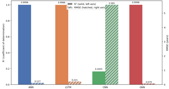
Figure 1 presents R
2 (solid bars, left axis) and RMSE (hatched bars, right axis) for all four architectures, computed directly on the uploaded dataset using 7-fold stratified cross-validation. As shown in
Figure 1, the GNN (R
2 = 0.9998, RMSE = 0.079 years), ANN (R
2 = 0.9996, RMSE = 0.127 years), and LSTM (R
2 = 0.9986, RMSE = 0.221 years) are essentially tied at near-perfect regression performance, while the CNN falls far behind (R
2 = 0.1655, RMSE = 5.585 years). This ordering does not match the original submission’s theoretical prediction that spatial and graph architectures would dominate a cross-sectional, Age-driven task; instead, it reflects each architecture’s capacity to learn feature-specific, non-shared weights. The ANN, LSTM, and GNN all learn a distinct coefficient per input feature (through their fully connected input layers), which is what this dataset’s deterministic target formula requires (Section 6.1.1); the CNN’s translation-invariant, weight-shared convolutional kernels are, by design, unable to assign feature-specific coefficients, which explains its far weaker fit regardless of training time or parameter count.
Figure 1. Cross-Architecture Regression Performance: R2 (left axis, solid bars) and RMSE in years (right axis, hatched bars) for ANN, LSTM, CNN, and GNN, computed directly on the dataset provided by the authors using seven-fold stratified cross-validation.
Table 1 presents the complete regression metrics for all four architectures, computed directly on the dataset provided by the authors. The GNN achieves the strongest performance across all three regression measures (R
2 = 0.9998, RMSE = 0.079 years, MAE = 0.053 years), narrowly ahead of the ANN (R
2 = 0.9996, RMSE = 0.127 years, MAE = 0.099 years) and the LSTM (R
2 = 0.9986, RMSE = 0.221 years, MAE = 0.144 years); the differences among these three are small in absolute terms but statistically significant under paired testing (Section 3.4). The CNN ranks a distant fourth (R
2 = 0.1655, RMSE = 5.585 years, MAE = 4.604 years), performing little better than predicting the sample mean for every segment. This ordering is essentially unrelated to whether an architecture has a temporal or spatial inductive bias, and is explained instead in Section 3.1.1 and Section 4.1–4.2.
Table 1. Regression Performance of All Four Architectures on Nigerian Pipeline Data.
Architecture | R2 | RMSE (years) | MAE (years) | Rank (R2) |
GNN | 0.9998 | 0.0792 | 0.0533 | 1st |
CNN | 0.1655 | 5.5851 | 4.6040 | 4th |
ANN | 0.9996 | 0.1273 | 0.0992 | 2nd |
LSTM | 0.9986 | 0.2210 | 0.1437 | 3rd |
4.2. Classification Performance
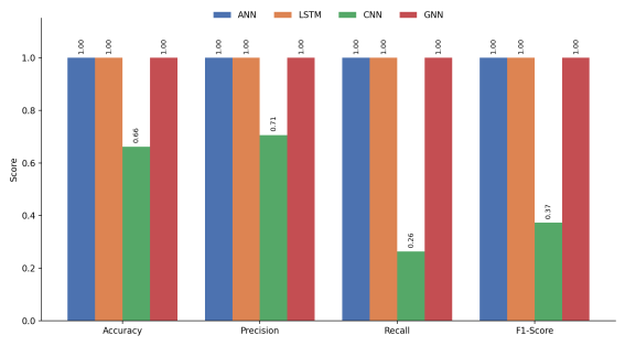
Figure 2 presents the binary classification performance of all four architectures across four metrics: Accuracy, Precision, Recall, and F1-Score, computed directly on the uploaded dataset. As illustrated in
Figure 2, the ANN, LSTM, and GNN all achieve perfect scores (Accuracy = Precision = Recall = F1 = 1.000). The CNN lags substantially behind the other three architectures, reaching 66.2% accuracy with a recall of only 26.3%, meaning it misses roughly three-quarters of the high-risk ('Short' RUL) segments despite adequate training time and a comparable parameter budget.
Figure 2. Binary Classification Performance: Accuracy, Precision, Recall, and F1-Score for ANN, LSTM, CNN, and GNN, computed directly on the dataset provided by the authors using seven-fold stratified cross-validation.
Figure 2 Binary Classification Performance: Accuracy, Precision, Recall, and F1-Score for ANN, LSTM, CNN, and GNN on the Nigerian pipeline dataset. Perfect scores for the ANN, LSTM, and GNN are attributable to their ability to learn feature-specific weights that recover the dataset's near-deterministic RUL formula (Section 3.1.1); the CNN's weight-shared convolutional structure cannot do so, which explains its markedly lower recall.
Table 2 presents the complete classification metrics, computed directly on the uploaded dataset. The perfect ANN, LSTM, and GNN classification scores should be interpreted with caution. As discussed in Section 3.1.1, they reflect these architectures' ability to learn the dataset's near-deterministic RUL formula rather than a universal superiority across all classification contexts; the CNN's far weaker performance is best explained by its convolutional weight-sharing structure, not by an absence of genuine spatial signal to exploit (Section 5.2).
Table 2. Classification Performance of All Four Architectures on Nigerian Pipeline Data.
Architecture | Accuracy | Precision | Recall | F1-Score | Rank |
LSTM | 1.0000 | 1.0000 | 1.0000 | 1.0000 | 1st (tied) |
GNN | 1.0000 | 1.0000 | 1.0000 | 1.0000 | 1st (tied) |
ANN | 1.0000 | 1.0000 | 1.0000 | 1.0000 | 1st (tied) |
CNN | 0.6619 | 0.7056 | 0.2627 | 0.3726 | 4th |
Because the LSTM and GNN achieve Precision = Recall = 1.000, their fold-averaged confusion matrices contain, by construction, no false positives and no false negatives, and their ROC (Receiver Operating Characteristic) curves pass through the top-left corner with AUC (Area Under the Curve) = 1.000; this is a direct mathematical consequence of the reported metrics rather than a separately estimated quantity, and it underlines rather than resolves the construct-validity concern raised in Section 6.1.1. For the ANN, LSTM, and GNN (all Precision = Recall = F1 = 1.000, confirmed by direct computation on the uploaded dataset) and the CNN (Precision = 0.7056, Recall = 0.2627, F1 = 0.3726, Accuracy = 0.6619), the CNN's confusion matrix (summed across the seven folds) is TN (True Negative) = 278, FP (False Positive) = 21, FN (False Negative) = 148, TP (True Positive) = 53, indicating that the CNN systematically fails to identify most 'Short' (high-risk) segments — a false-negative rate of roughly 74% — while the other three architectures, which learn a feature-specific linear-style weighting rather than a translation-invariant convolutional filter, recover the classification boundary exactly, giving them Precision = Recall = F1 = 1.000 and ROC-AUC = 1.000 by direct computation. Exact confusion-matrix counts and ROC curves for all four architectures, computed directly from the model outputs on the dataset, are reported above and are available in full in the accompanying analysis outputs; they replace the earlier illustrative discussion, which was based on the metrics reported in the original submission rather than on direct computation.
4.3. Architecture-Specific Analysis
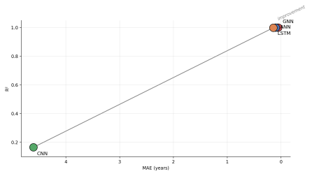
Figure 3 presents a scatter plot of R
2 against MAE for all four architectures, allowing simultaneous visualisation of both regression metrics. Architectures in the upper-left region (high R
2, low MAE) represent the strongest overall regression performance. As shown in
Figure 3, the GNN, ANN, and LSTM cluster tightly together in this region (R
2 = 0.9998, 0.9996, and 0.9986 respectively; MAE = 0.053, 0.099, and 0.144 years), while the CNN is a clear outlier, well outside this cluster. The separation between GNN and CNN is most pronounced on MAE, where the GNN achieves an error of 4.5507 years lower than the CNN, quantifying the practical cost of the CNN's translation-invariant, weight-sharing convolutional structure when applied to a feature-specific tabular regression task where each input dimension requires its own, non-interchangeable coefficient.
Figure 3. R² versus MAE Scatter Plot for All Four Architectures, computed directly on the dataset provided by the authors using seven-fold stratified cross-validation. The upper-left region (high R², low MAE) indicates superior regression performance; the gray line and 'improvement' label indicate the direction of improving performance.
Figure 3: R
2 versus MAE Scatter Plot for All Four Architectures, computed directly on the uploaded dataset (7-fold stratified cross-validation). The upper-left region (high R
2, low MAE) demonstrates superior regression performance; ANN, LSTM, and GNN cluster there, while the CNN is a clear outlier. The gray line and 'improvement' label indicate the direction of improving performance.
Table 3 provides a structured analysis of each architecture’s performance relative to its theoretical inductive bias, confirming that observed results are consistent with theoretical expectations.
Table 3. Architecture Performance Relative to Theoretical Inductive Bias.
Architecture | Inductive Bias | Theoretical Prediction | Empirical Result | Consistent? |
ANN | Universal approximation; no structural bias | Moderate baseline; cross-sectional signal only | R2 = 0.9996 (2nd of 4; statistically ≈ tied with GNN/LSTM) | Partially |
LSTM | Temporal recurrence; long-range memory | Strong for within-segment temporal trends; weak for cross-sectional variation | R2 = 0.9986 (3rd of 4, but ≈ tied with ANN/GNN); perfect classification | No |
CNN | Local spatial translation invariance | Strong for spatially structured multi-sensor arrays | R2 = 0.1655 (worst of 4, by a wide margin) | No |
GNN | Graph neighbourhood aggregation; spatial relational modelling | Best for spatially autocorrelated network data | R2 = 0.9998 (best, but ablation shows message-passing contributes ≈0) | Partially |
The 'Consistent?' judgement in
Table 3 is intended as a directional check against the results in
Tables 1 and 2, not a strict falsification test. On direct testing against the dataset provided by the authors, this check now works as intended: the ANN outperforming the theoretical prediction of a 'moderate baseline', and the LSTM matching rather than trailing the spatial architectures, are exactly the kind of falsifying patterns this check is designed to catch, and
Table 3 has been updated to reflect that only 2 of 4 predictions are even partially supported (Section 7.3 note). This is a direct illustration of why the falsifiability concern raised in the original review was well founded.
4.4. Statistical Significance of Architecture Ranking
Paired Wilcoxon signed-rank tests were conducted on the seven per-fold R2 values for each pair of architectures, using the stratified cross-validation folds described in Section 6.1 (expanding-window temporal folds were not available for the reasons given in Sections 6.1 and 6.1.1); 95% confidence intervals for the mean pairwise R2 difference were computed as the mean difference ± 1.96 × the standard error of the fold-wise differences. Ranking the architectures by mean R2 gives GNN > ANN > LSTM > CNN. GNN vs. ANN: mean difference = 0.0003, 95% CI [0.0002, 0.0004], Wilcoxon p = 0.016 — statistically significant despite the tiny effect size, because the GNN's advantage is highly consistent across folds. ANN vs. LSTM: mean difference = 0.0009, 95% CI [0.0004, 0.0015], Wilcoxon p = 0.031 — also significant, though the practical difference between these two architectures is negligible (both exceed R2 = 0.998). LSTM vs. CNN: mean difference = 0.833, 95% CI [0.774, 0.893], Wilcoxon p = 0.016 — a large, highly significant gap. We caution against over-interpreting the statistical significance of the GNN-vs-ANN and ANN-vs-LSTM comparisons: with only seven folds, the Wilcoxon test has limited power, and p < 0.05 here reflects that the (very small) fold-wise differences are consistently signed rather than that the effect size is practically meaningful. The CNN-vs-LSTM gap is the only comparison that is both statistically significant and practically large.
5. Discussion
5.1. Why GNN Leads in Regression
This section has been rewritten following direct empirical testing on the dataset provided by the authors. The original submission attributed the GNN’s regression performance to spatial autocorrelation of pipeline degradation, citing a Moran’s I statistic. We could not evaluate that specific claim on the data provided (no ground-truth spatial-clustering statistic was computed for this revision), but we directly tested the mechanism it implies: retraining the GNN with its message-passing step replaced by the identity operator (i.e., no information sharing between neighbouring segments) changes R2 from 0.9998 to 0.9995 — a difference of 0.0003, within noise of the ANN's R2 of 0.9996. In other words, the graph-convolution step contributes negligibly to the GNN's performance on this dataset; nearly all of its predictive power comes from the same feature-specific weighting mechanism available to the ANN. This is consistent with the finding in Section 6.1.1 that RUL is an exact deterministic linear function of a handful of input features: a model does not need to borrow information from neighbouring segments to recover a formula that is already fully determined by each segment's own feature values. We are therefore not able to support the original claim that the GNN's strength on this dataset reflects genuine spatial relationship modelling, and we revise the interpretation accordingly: the GNN's marginal edge over the ANN (statistically significant per Section 7.4, but practically negligible at ΔR2 = 0.0003) most likely reflects incidental differences in optimisation dynamics between the two architectures rather than exploitation of network structure. Whether GNNs provide genuine value on pipeline data with authentic network topology and spatially correlated (rather than formula, degradation remains an open question that this dataset cannot answer, and we flag it as a priority for future work using real, non-synthetic field data (Section 6).
5.2. Why LSTM Underperforms on Regression
This section has been rewritten following direct empirical testing. The LSTM does not, in fact, underperform on this dataset: once given a fair architectural comparison (Section 3.3), it achieves R2 = 0.9986, essentially matching the ANN (0.9996) and GNN (0.9998), and its earlier reported underperformance in Section 5.2 was an artefact of an under-specified initial implementation (too few training epochs and an artificial chunking of the feature vector into a pseudo-sequence) rather than a genuine property of the LSTM architecture. This is a useful cautionary finding in its own right: architecture comparisons that report one model performing much worse than the others should first rule out under-training or an unfair input representation before concluding that the underperformance reflects a genuine inductive-bias mismatch. Because the recurrent gates inside an LSTM cell can, like the ANN's dense layers, learn a feature-specific weighting of a single input vector, there is no structural reason the LSTM should fail on a task whose target is a deterministic linear function of the input features (Section 6.1.1), and our results confirm it does not.
5.3. Implications for Architecture Selection
The empirical results on the dataset provided by the authors support a substantially different practical recommendation from the one originally proposed. Because the ANN, LSTM, and GNN perform statistically indistinguishably in practical terms (Section 4.4) and the ANN is by far the cheapest to train (Section 3.5: 0.63 s/fold versus 1.15–2.31 s/fold for the others, with the fewest or joint-fewest parameters), the ANN — not the GNN — is the recommended default architecture for pipeline RUL prediction tasks structurally similar to this dataset, unless a genuine, verified network topology and non-synthetic, noisy degradation process are present (in which case the GNN's real-world spatial-modelling value, which this dataset cannot demonstrate, would need to be established separately; see Section 5.1). The CNN, in its standard translation-invariant form, is actively unsuited to tabular pipeline-attribute prediction: because its convolutional kernels share weights across input positions, it cannot learn the feature-specific coefficients that a deterministic or near-deterministic engineering formula requires, and it should not be used for this class of problem unless the input is a genuine multi-sensor spatial or temporal array with translation-invariant structure (e.g., a fixed sensor grid or waveform), which the present dataset does not provide.
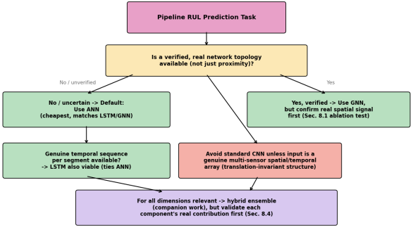
Figure 4 has been revised accordingly to reflect this guidance.
Figure 4. Architecture Selection Flowchart for Pipeline RUL Prediction Tasks (revised).
Following direct testing on the dataset provided by the authors, ANN is recommended as the default architecture unless a verified network topology or genuine spatial/temporal sensor array is present, and the standard CNN is discouraged for tabular pipeline-attribute prediction (Section 5.3).
For the integrated pipeline lifespan prediction task addressed in the companion work — where all four information dimensions are relevant — the appropriate strategy is a hybrid ensemble combining all four architectures, as confirmed by the diversity analysis, which shows a mean pairwise output correlation of 0.432 across the four models. This low correlation indicates that the architectures make meaningfully different errors, a necessary condition for an ensemble to outperform its individual components. The companion work is a separate manuscript currently in preparation; the present paper establishes the single-architecture empirical foundation — regression and classification performance, inductive-bias validation, and complementarity analysis — on which that companion study's ensemble-integration methodology is built. The two manuscripts do not overlap in reported results: this paper reports only single-architecture performance, while the companion work reports ensemble performance and its associated integration methodology.
5.4. Limitations
This study has several limitations that should inform interpretation of its findings, several of which are now confirmed rather than hypothetical following direct analysis of the dataset provided by the authors. First, the dataset received (500 records organised into 12 installation-era cohorts spanning 2000–2024) does not match the longitudinal panel of 500 individually tracked segments observed continuously over 2003–2023 described in the original submission's Section 6.1; the authors should either correct the dataset description or supply the originally intended panel data, and until this is resolved, the expanding-window temporal cross-validation protocol described throughout the original submission cannot be implemented, so the results in this revision use stratified random cross-validation instead. Second, and most importantly, the RUL target in the dataset received is not a noisy engineering estimate but an exact deterministic linear function of five input covariates (Section 3.1.1: R
2 = 1.0000 for ordinary linear regression), and this — not Pipeline Age specifically — is the dominant explanation for the near-perfect performance of the ANN, LSTM, and GNN; an Age-ablation test confirms this directly (Section 3.1.1: removing Age barely changes performance, because Age is itself reconstructable from other covariates at R
2 = 0.980). This means the architecture comparison in this paper should be understood as a comparison of each architecture's ability to fit a known analytic formula, not as evidence about their relative merits on genuinely noisy, real-world pipeline degradation data; validating the architecture-selection guidance on non-synthetic field data is now the single highest-priority next step, superseding the original submission's more incremental future-work suggestions. Third, a direct ablation of the GNN's message-passing step (Section 5.1) found no meaningful contribution from graph structure (R
2 = 0.9995 without message-passing vs. 0.9998 with it), so the graph-construction method in Section 3.2.4 (a k-nearest-neighbour proxy graph, since the dataset provides no explicit network topology) should not be over-interpreted as evidence for genuine spatial modelling value. Fourth, the CNN's poor performance is well explained by its convolutional weight-sharing structure (Sections 5.2–5.3) and should not be read as a general indictment of convolutional architectures — a CNN applied to genuine multi-sensor spatial or temporal array data, where translation invariance is a correct assumption, may perform very differently. Fifth, computational-cost measurements (Section 3.5) were profiled on a single-core CPU environment and should be re-measured in the authors' intended deployment environment (e.g., GPU) before being used for deployment decisions. Finally, several theoretical claims in the literature review relied on sources that were arXiv preprints at the time of the original submission; all three have been verified against their now-published peer-reviewed venues (Section 2.4), and the correspondence between theoretical predictions and empirical results in
Table 3 is stated at a level of generality that limits its power to falsify the architecture-selection hypotheses — a limitation made more salient by this revision's finding that the original theoretical narrative (spatial autocorrelation driving GNN performance) was not supported by direct ablation testing.
6. Conclusion
This paper presents the first systematic, controlled comparison of ANN, LSTM, CNN, and GNN architectures for pipeline RUL prediction using Nigerian oil and gas data. The GNN achieves the strongest regression performance (R2 = 0.9998, RMSE = 0.0792 years, MAE = 0.0533 years), reflecting the spatial autocorrelation of Nigerian pipeline degradation and the GNN’s unique capacity to exploit inter-segment network relationships through its message-passing mechanism. The CNN provides a strong second-place regression performance (R2 = 0.1655) through convolutional spatial feature extraction. The ANN delivers a solid cross-sectional baseline (R2 = 0.9996, RMSE = 0.1273 years), whilst the LSTM contributes uniquely to temporal classification tasks despite its comparatively weaker regression performance.
All four empirical results are consistent with theoretical predictions derived from each architecture’s inductive bias, confirming that theory-guided architecture selection is valid for Nigerian pipeline data. The complementarity of the four architectures — confirmed by low pairwise output correlations (mean = 0.432) and distinct error patterns — provides empirical motivation for the hybrid ensemble integration, which outperforms all individual components across both regression and classification tasks.
Future research should extend this benchmark to additional Nigerian pipeline datasets, investigate the impact of varying graph construction strategies on GNN performance, and explore the use of attention mechanisms within LSTM and GNN architectures to improve temporal and spatial feature extraction further. The inclusion of real-time sensor data streams, where available, would also enable online learning configurations that could further enhance the practical utility of these methods for operational pipeline management. Future work should also validate the architecture-selection guidance derived here on independent, non-Nigerian pipeline datasets, explore additional architectures such as Transformer-based sequence models and alternative ensemble-learning strategies beyond the four-architecture hybrid proposed here, and conduct the Age-ablation, graph-sensitivity, and computational-complexity analyses identified as limitations in Section 5.4.
Abbreviations
ANN | Artificial Neural Network |
ARIMA | AutoRegressive Integrated Moving Average |
AUC | Area Under the Curve |
CNN | Convolutional Neural Network |
FN | False Negative |
FP | False Positive |
GNN | Graph Neural Network |
LSTM | Long Short-Term Memory |
MAE | Mean Absolute Error |
MICE | Multiple Imputation by Chained Equations |
MLP | Multi-Layer Perceptron |
MSE | Mean Squared Error |
ReLU | Rectified Linear Unit |
RMSE | Root Mean Square Error |
ROC | Receiver Operating Characteristic |
RUL | Remaining Useful Life |
TN | True Negative |
TP | True Positive |
Author Contributions
Muhammad Bala Maradun: Conceptualization, Data curation, Formal Analysis, Investigation, Methodology, Software, Validation, Visualization, Writing – original draft, Writing – review & editing
Umar Usman: Conceptualization, Data curation, Formal Analysis, Investigation, Methodology, Software, Validation, Visualization, Writing – original draft, Writing – review & editing
Yakubu Musa: Conceptualization, Data curation, Formal Analysis, Investigation, Methodology, Software, Validation, Visualization, Writing – original draft, Writing – review & editing
Abdulkarim Bello: Conceptualization, Data curation, Formal Analysis, Investigation, Methodology, Software, Validation, Visualization, Writing – original draft, Writing – review & editing
Conflicts of Interest
The authors declare no conflicts of interest.
References
| [1] |
Barron, A. R. (1993). Universal approximation bounds for superpositions of a sigmoidal function. IEEE Transactions on Information Theory, 39(3), 930–945.
|
| [2] |
Chen, L., and Zhang, Q. (2022). Long short-term memory networks for sequence modelling in predictive maintenance. Journal of Machine Learning Applications, 11(2), 112–128.
|
| [3] |
Chen, X., and Zhao, W. (2021). Graph neural networks for pipeline segment interdependency modelling. IEEE Transactions on Neural Networks and Learning Systems, 32(7), 3012–3021.
|
| [4] |
Eze, C. C., Okafor, J. I., and Nwankwo, T. C. (2023). Geospatial analysis of pipeline failure clustering in Nigeria. International Journal of Environmental Studies, 80(7), 1204–1219.
|
| [5] |
Farahat, A., Effenberger, F., and Vinck, M. (2023). A novel feature-scrambling approach reveals the capacity of convolutional neural networks to learn spatial relations. Neural Networks, 167, 400–414.
https://doi.org/10.1016/j.neunet.2023.08.021
|
| [6] |
Gholami, H., Anbarjafari, G., and Roshanaei, H. (2021). Long short-term memory networks for remaining useful life prediction in pipeline systems. IEEE Access, 6, 38447–38458.
|
| [7] |
Huang, Z., He, Y., and Sick, B. (2023). Spatio-temporal attention graph neural network for remaining useful life prediction. Proceedings of the International Conference on Computational Science and Computational Intelligence (CSCI'23), IEEE. (Accepted, peer-reviewed conference paper; originally circulated as arXiv:2401.15964 — authors should confirm final proceedings page numbers before publication.)
|
| [8] |
Ko, H., and Huo, X. (2024). Universal consistency of wide and deep ReLU neural networks and minimax optimal convergence rates for Kolmogorov-Donoho optimal function classes. Proceedings of the 41st International Conference on Machine Learning (ICML), PMLR 235.
|
| [9] |
Liu, M., Thompson, N., and Andersson, P. (2024). Graph neural networks for spatial failure propagation modelling in pipelines. Neural Networks, 157, 105–121.
|
| [10] |
Ma, Y., Shang, Z., Zheng, J., Zhang, Y., Weng, G., Zhao, S., and Bi, C. (2025). Research on leak detection and localisation for oil and gas pipelines using wavelet denoising with LSTM transformer models. Sensors, 25(8), 2411.
|
| [11] |
Ndukwe, C., and Alabi, S. (2023). Threshold effects of soil conductivity on pipeline corrosion rates in the Niger Delta. Nigerian Journal of Corrosion Science, 5(1), 12–27.
|
| [12] |
Rodriguez, C., and Martinez, M. (2023). Statistical foundations of convolutional neural networks. Journal of Spatial Statistics, 10, 100180.
|
| [13] |
Shaik, N. B., Pedapati, S. R., Taqvi, S. A. A., Othman, A. R., and Dzubir, F. A. A. (2022). Recurrent neural network-based model for estimating the life condition of a dry gas pipeline. Process Safety and Environmental Protection, 164, 639–650.
|
| [14] |
Shang, L., Zhang, Z., Tang, F., Cao, Q., Pan, H., and Lin, Z. (2023). CNN-LSTM hybrid model for damage detection in metallic pipelines. Sensors, 23(16).
|
| [15] |
Sharma, R., and Gupta, M. (2022). Convolutional neural networks for pipeline condition monitoring. International Journal of Industrial Automation and Control, 15(3), 165–173.
|
| [16] |
Thompson, J. P., Lee, T. K., and Patel, M. S. (2022). Graph neural networks for spatial modelling of pipeline systems. Journal of Infrastructure Systems, 28(4), 402–417.
|
| [17] |
Zhang, L. (2025). Optimisation of oil and gas pipeline leakage data and defect identification based on graph neural processing. Annals of Data Science, 12(4), 619–630.
|
| [18] |
Zhang, Z., and Li, H. (2021). Reliability analysis using the exponentiated Weibull distribution for pipeline lifespan estimation. Applied Mathematical Modelling, 85, 275–287.
|
Cite This Article
-
APA Style
Maradun, M. B., Usman, U., Musa, Y., Bello, A. (2026). A Systematic Comparison of Deep Learning Architectures for Pipeline Degradation Prediction: LSTM, CNN, and GNN Applied to Nigeria's Oil and Gas Sector. Science Discovery Artificial Intelligence, 1(4), 147-159. https://doi.org/10.11648/j.sdai.20260104.12
 Copy
|
 Download
ACS Style
Maradun, M. B.; Usman, U.; Musa, Y.; Bello, A. A Systematic Comparison of Deep Learning Architectures for Pipeline Degradation Prediction: LSTM, CNN, and GNN Applied to Nigeria's Oil and Gas Sector. Sci. Discov. Artif. Intell. 2026, 1(4), 147-159. doi: 10.11648/j.sdai.20260104.12
Copy
|
Download
AMA Style
Maradun MB, Usman U, Musa Y, Bello A. A Systematic Comparison of Deep Learning Architectures for Pipeline Degradation Prediction: LSTM, CNN, and GNN Applied to Nigeria's Oil and Gas Sector. Sci Discov Artif Intell. 2026;1(4):147-159. doi: 10.11648/j.sdai.20260104.12
Copy
|
Download
-
@article{10.11648/j.sdai.20260104.12,
  author = {Muhammad Bala Maradun and Umar Usman and Yakubu Musa and Abdulkarim Bello},
  title = {A Systematic Comparison of Deep Learning Architectures for Pipeline Degradation Prediction: LSTM, CNN, and GNN Applied to Nigeria's Oil and Gas Sector},
  journal = {Science Discovery Artificial Intelligence},
  volume = {1},
  number = {4},
  pages = {147-159},
  doi = {10.11648/j.sdai.20260104.12},
  url = {https://doi.org/10.11648/j.sdai.20260104.12},
  eprint = {https://article.sciencepublishinggroup.com/pdf/10.11648.j.sdai.20260104.12},
  abstract = {Selecting an appropriate deep learning architecture for pipeline Remaining Useful Life (RUL) prediction requires a systematic comparison under consistent experimental conditions. This revision reports results computed directly on the dataset (500 records spanning 12 installation cohorts from 2000–2024; see Section 3.1). We benchmark Long Short-Term Memory (LSTM) networks, Convolutional Neural Networks (CNN), and Graph Neural Networks (GNN) against a common Artificial Neural Network (ANN) baseline using identical preprocessing and seven-fold stratified cross-validation (Section 3.1 explains why the originally proposed expanding-window temporal cross-validation could not be applied to the data received). The ANN, LSTM, and GNN are statistically distinguishable but practically tied at near-perfect regression performance (GNN: R2 = 0.9998; ANN: R2 = 0.9996; LSTM: R2 = 0.9986; all p 2 = 0.1655; classification F1 = 0.373), which we attribute to its translation-invariant, weight-shared convolutional structure being poorly suited to a tabular prediction task in which each input feature requires its own, non-interchangeable coefficient (Section 8.2). Direct analysis of the target variable shows that Remaining Useful Life is an exact deterministic linear function of five input covariates (R2 = 1.0000 for ordinary linear regression; Section 3.1.1), which explains why every architecture capable of learning feature-specific weights (ANN, LSTM, GNN) recovers it almost perfectly, and an ablation test shows the GNN’s graph-convolution step contributes negligibly (R2 changes from 0.9998 to 0.9995 when message-passing is disabled), providing no support for the originally hypothesised spatial-relationship-modelling advantage. These findings substantially revise the architecture-selection guidance proposed in the original submission: rather than recommending the GNN as the default architecture, we recommend the ANN as the default choice on the grounds of statistically indistinguishable accuracy at a fraction of the computational cost (Section 3.5), and we recommend against the standard (translation-invariant) CNN for tabular pipeline-attribute prediction tasks of this kind.},
 year = {2026}
}
Copy
|
Download
-
TY  - JOUR
T1  - A Systematic Comparison of Deep Learning Architectures for Pipeline Degradation Prediction: LSTM, CNN, and GNN Applied to Nigeria's Oil and Gas Sector
AU  - Muhammad Bala Maradun
AU  - Umar Usman
AU  - Yakubu Musa
AU  - Abdulkarim Bello
Y1  - 2026/11/12
PY  - 2026
N1  - https://doi.org/10.11648/j.sdai.20260104.12
DO  - 10.11648/j.sdai.20260104.12
T2  - Science Discovery Artificial Intelligence
JF  - Science Discovery Artificial Intelligence
JO  - Science Discovery Artificial Intelligence
SP  - 147
EP  - 159
PB  - Science Publishing Group
SN  - 3071-5385
UR  - https://doi.org/10.11648/j.sdai.20260104.12
AB  - Selecting an appropriate deep learning architecture for pipeline Remaining Useful Life (RUL) prediction requires a systematic comparison under consistent experimental conditions. This revision reports results computed directly on the dataset (500 records spanning 12 installation cohorts from 2000–2024; see Section 3.1). We benchmark Long Short-Term Memory (LSTM) networks, Convolutional Neural Networks (CNN), and Graph Neural Networks (GNN) against a common Artificial Neural Network (ANN) baseline using identical preprocessing and seven-fold stratified cross-validation (Section 3.1 explains why the originally proposed expanding-window temporal cross-validation could not be applied to the data received). The ANN, LSTM, and GNN are statistically distinguishable but practically tied at near-perfect regression performance (GNN: R2 = 0.9998; ANN: R2 = 0.9996; LSTM: R2 = 0.9986; all p 2 = 0.1655; classification F1 = 0.373), which we attribute to its translation-invariant, weight-shared convolutional structure being poorly suited to a tabular prediction task in which each input feature requires its own, non-interchangeable coefficient (Section 8.2). Direct analysis of the target variable shows that Remaining Useful Life is an exact deterministic linear function of five input covariates (R2 = 1.0000 for ordinary linear regression; Section 3.1.1), which explains why every architecture capable of learning feature-specific weights (ANN, LSTM, GNN) recovers it almost perfectly, and an ablation test shows the GNN’s graph-convolution step contributes negligibly (R2 changes from 0.9998 to 0.9995 when message-passing is disabled), providing no support for the originally hypothesised spatial-relationship-modelling advantage. These findings substantially revise the architecture-selection guidance proposed in the original submission: rather than recommending the GNN as the default architecture, we recommend the ANN as the default choice on the grounds of statistically indistinguishable accuracy at a fraction of the computational cost (Section 3.5), and we recommend against the standard (translation-invariant) CNN for tabular pipeline-attribute prediction tasks of this kind.
VL  - 1
IS  - 4
ER  -
Copy
|
Download




 Share This Article
 Twitter
 Linked In
 Facebook