Research Article | | Peer-Reviewed

Comparative GIS-Based Landslide Susceptibility and Relative Risk Assessment Using Frequency Ratio, Shannon Entropy and Statistical Information Index Models

Received: 25 June 2026     Accepted: 6 July 2026     Published: 24 July 2026
Views:       Downloads:
Abstract

Landslides are recurrent geomorphic hazards in the Nepal Himalaya, where fragile geology, steep terrain, monsoonal rainfall and expanding road construction increase slope instability. This study assesses landslide susceptibility and relative risk in Tamakoshi Rural Municipality, Dolakha, Nepal, by comparing three GIS-based bivariate models: frequency ratio (FR), Shannon entropy (SE) and statistical information index (SII). A landslide inventory of 121 events was prepared from Google Earth imagery, satellite-image interpretation and field verification, and divided into 70% training and 30% validation subsets. Ten conditioning factors were analysed at 30 m spatial resolution: slope, aspect, curvature, elevation, topographic wetness index, lithology, soil type, land use/land cover, distance from roads and distance from rivers. Model discrimination was evaluated using receiver operating characteristic-area under the curve analysis. Landslides were concentrated on steep, mid-elevation slopes, particularly within 250 m of rivers and 100 m of roads, indicating the influence of fluvial undercutting, road excavation and drainage disturbance. SII produced the highest success and prediction AUC values (0.654 and 0.628), followed by FR (0.645 and 0.623) and SE (0.634 and 0.613), although all three models showed only modest discrimination. An AHP-based exposure–vulnerability index was prepared from settlement, population, road, school, hospital and temple indicators. The resulting relative risk zonation identified approximately 15% of the municipality as high or very high risk, mainly in wards 1, 3 and 5. The findings provide a spatial basis for field prioritization, risk-sensitive land-use planning and local disaster risk reduction.

Published in American Journal of Applied Scientific Research (Volume 12, Issue 3)
DOI 10.11648/j.ajasr.20261203.13
Page(s) 81-102
Creative Commons

This is an Open Access article, distributed under the terms of the Creative Commons Attribution 4.0 International License (http://creativecommons.org/licenses/by/4.0/), which permits unrestricted use, distribution and reproduction in any medium or format, provided the original work is properly cited.

Copyright

Copyright © The Author(s), 2026. Published by Science Publishing Group

Keywords

AHP, Lesser Himalaya, Mountain Hazards, ROC-AUC, Spatial Modelling, Terrain Analysis, Vulnerability Assessment

1. Introduction
Landslides are among the most frequent and destructive geomorphic hazards in mountainous regions. They threaten settlements, roads, agricultural land, forests, drainage systems and public infrastructure through the downslope movement of rock, debris and soil. In the Himalayan region, landslide occurrence is controlled by the interaction of active tectonics, steep relief, fractured lithology, intense monsoonal rainfall, deeply incised river systems and increasing human disturbance . Nepal is particularly exposed to landslide hazards because most of the country consists of hill and mountain terrain where elevation changes rapidly over short horizontal distances. The young and tectonically active Himalayan geology, combined with weak rock mass, complex geomorphology and seasonal rainfall, creates naturally unstable slope conditions .
Anthropogenic activities further intensify slope instability in Nepal. Road excavation, unplanned slope cutting, vegetation removal, agricultural terracing, land-use modification and inadequate drainage management frequently disturb natural slope equilibrium . Rural road construction is especially important because road cuts often over-steepen slopes, expose weak materials, redirect surface runoff and reduce toe support. Such conditions increase the probability of shallow landslides and road-side failures during intense rainfall events . Landslide susceptibility expresses the relative spatial likelihood of landslide occurrence under specific terrain and environmental conditions. It differs from landslide hazard, which also requires information on temporal probability, frequency or magnitude, and from risk, which additionally considers exposed elements and vulnerability . Although susceptibility maps do not estimate exact timing or expected loss, they are valuable planning tools because they identify areas where future slope failures are more likely than elsewhere. In data-limited mountain regions, Geographic Information Systems (GIS), remote sensing and statistical modelling provide an effective framework for preparing landslide inventories, deriving conditioning factors and producing spatial susceptibility assessments .
Several approaches have been developed for landslide susceptibility mapping, including heuristic, physically based, statistical, machine-learning and hybrid methods . However, bivariate statistical methods remain useful for municipal-scale studies because they are transparent, reproducible, computationally efficient and easy to communicate to local planners and disaster-management authorities. These methods are particularly suitable where detailed geotechnical data, rainfall thresholds and long-term landslide records are limited. Frequency Ratio (FR), Shannon Entropy (SE) and Statistical Information Index (SII) are widely applied bivariate models for landslide susceptibility assessment. FR evaluates the relationship between landslide occurrence and each class of a conditioning factor by comparing landslide density with area density . SE applies information theory to estimate the relative contribution of conditioning factors and derive objective weights . SII, also known as the information value method, assigns positive or negative weights to factor classes based on the ratio between class-specific landslide density and overall landslide density. The performance of these models is site-dependent because it is influenced by landslide inventory quality, factor selection, factor classification, spatial resolution and local geomorphic conditions.
Recent studies in Nepal have demonstrated the continued relevance of bivariate modelling for landslide susceptibility assessment. Comparative studies using FR, weights of evidence, SE and information value models show that the best-performing model varies according to geology, terrain, landslide inventory and study scale . However, many local-scale studies focus mainly on susceptibility mapping and do not sufficiently integrate the spatial distribution of settlements, roads and public services into risk-oriented outputs. In addition, comparative evaluation of FR, SE and SII remains limited in the Lesser Himalayan setting of central-eastern Nepal. Tamakoshi Rural Municipality of Dolakha District contains steep and dissected slopes, fractured rocks, deeply incised river valleys, expanding rural roads, agricultural terraces and settlements located close to unstable terrain. Landslides commonly affect road-cut sections, river valleys, cultivated land, forested hillslopes and geologically weak zones. Therefore, the municipality provides an appropriate setting for testing interpretable susceptibility models and linking the best-performing output with exposure-vulnerability indicators.
The aim of this study is to compare FR, SE and SII models for landslide susceptibility assessment and to prepare a relative landslide risk zonation map for Tamakoshi Rural Municipality. The specific objectives are: (i) to prepare a landslide inventory using Google Earth imagery, satellite-image interpretation and field verification; (ii) to analyze the relationship between landslide occurrence and selected conditioning factors; (iii) to compare FR, SE and SII models using success-rate and prediction-rate ROC-AUC values; and (iv) to integrate the best-performing susceptibility output with an AHP-based exposure-vulnerability index. The study is intended to support field prioritization, risk-sensitive land-use planning, infrastructure management and local disaster risk reduction.
2. Materials and Methods
2.1. Study Area
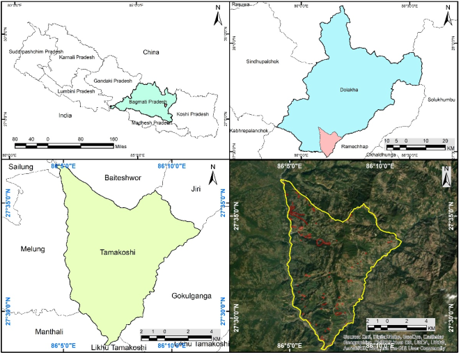
Tamakoshi Rural Municipality is located in Dolakha district of Bagmati Province, central-eastern Nepal, between 27°28′27″–27°36′47″ N and 86°04′22″–86°11′11″ E. The municipality lies within the Lesser Himalayan geological sequence and is located approximately 170 km northeast of Kathmandu. It is accessible through the Lamosangu–Ramechhap Highway and connected internally by rural roads. Elevation ranges from approximately 580 to 2240 m above sea level. The terrain is characterized by steep slopes, ridges, spurs, saddles, deeply incised valleys, alluvial terraces and colluvial deposits. The Tamakoshi River is the major drainage system, supported by several seasonal tributaries forming a dendritic drainage pattern. River undercutting, slope excavation and poor drainage management are major contributors to slope instability in the area.
The municipality is dominated by agricultural land and forest. Cultivated areas are mainly located in the central and southeastern parts, while forested areas are common in the northern and southwestern parts. Landslides occur in agricultural land, forests, grasslands, road-cut sections and river valleys, indicating the combined effect of natural and anthropogenic factors. The study area experiences tropical to temperate climatic conditions depending on elevation. Rainfall is mainly concentrated during the monsoon season, and annual rainfall ranges from about 1600 mm to 2000 mm. The location of the study area is shown in Figure 1.
Figure 1. Location map of Tamakoshi Rural Municipality.
2.2. Research Design and Methodological Workflow
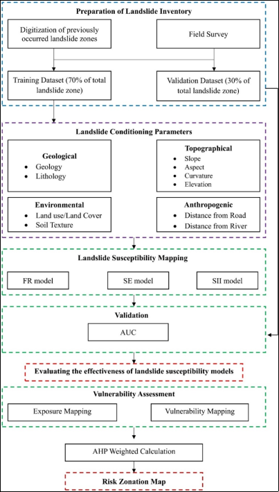
The study followed a GIS-based comparative framework for landslide susceptibility and relative risk assessment. The workflow included landslide inventory preparation, spatial data collection, conditioning-factor preparation, susceptibility modelling, validation, exposure-vulnerability assessment and relative risk zonation.
First, landslide polygons were identified using Google Earth imagery, satellite image interpretation and field verification. The inventory was divided into training and validation datasets. Ten conditioning factors were prepared and converted into a common raster format. Class-wise landslide and non-landslide pixel statistics were calculated by overlaying the training inventory with each conditioning-factor layer. These statistics were used to derive Frequency Ratio (FR), Shannon Entropy (SE) and Statistical Information Index (SII) weights. The resulting susceptibility maps were validated using Receiver Operating Characteristic-Area Under the Curve (ROC-AUC) analysis. Finally, the best-performing susceptibility output was combined with an AHP-based exposure-vulnerability index to generate the relative landslide risk zonation map. The methodological workflow is presented in Figure 2.
Figure 2. Methodological workflow for inventory preparation, susceptibility modelling, validation, exposure-vulnerability assessment and relative risk zonation.
2.3. Data Sources and Spatial Preprocessing
Both primary and secondary datasets were used in this study. Primary data included field observations, GPS-based checking of selected landslide locations and documentation of landslide characteristics. Secondary data included Digital Elevation Model (DEM), land use/land cover, geological data, soil type, road network, river network, settlement and population-related datasets. All spatial layers were projected to WGS 1984 UTM Zone 45N. Vector data were converted to raster format and all raster layers were aligned to a common 30 m × 30 m grid, spatial extent and cell origin. Resampling and alignment were completed before overlay analysis to ensure cell-by-cell compatibility.
Table 1. Data sources used in this assessment.

Data layer

Source

Scale or resolution

Landslide inventory

Google Earth imagery, satellite image interpretation and field survey

Polygon inventory

DEM

USGS Earth Explorer

30 m

Land use and land cover

ICIMOD portal

30 m

Geological data

Department of Mines and Geology, Nepal

1:50,000

Landsat-8 imagery

USGS Earth Explorer

30 m

Road network

Google Earth imagery and GIS digitization

Vector data

River network

Humanitarian Data Exchange and hydrological sources

Vector data

Soil type

FAO land resources database

Thematic data

Settlement data

Google Earth imagery and field verification

Vector data

Population distribution

Available population dataset

Raster or administrative data

2.4. Landslide Inventory Preparation
A landslide inventory is the fundamental input for data-driven landslide susceptibility modelling because it records the spatial distribution of previous slope failures . In this study, landslides were identified using Google Earth imagery, satellite image interpretation and field verification. Diagnostic features such as fresh scars, exposed soil or rock, disrupted drainage, displaced road sections, accumulation zones and surface-texture changes were used for landslide identification.
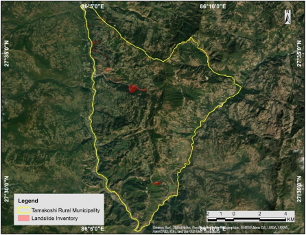
A total of 121 landslide locations were mapped. These included rockfalls, debris slides, shallow translational slides, creep movements and active or reactivated slope failures. Field verification confirmed several instability indicators, including crown cracks, tension cracks, seepage, slope bulging, road deformation and damage to agricultural land and retaining structures. The landslide inventory was divided into training and validation datasets. The training dataset consisted of 85 landslide locations, representing 70% of the total inventory, and contained 938 landslide raster cells. The remaining 36 landslide locations, representing 30% of the inventory, were used for independent validation. The landslide inventory map is shown in Figure 3.
Figure 3. Landslide inventory of Tamakoshi Rural Municipality prepared from image interpretation and field verification.
2.5. Landslide-Conditioning Factors
Ten landslide-conditioning factors were selected based on the geomorphic setting, field evidence, data availability and previous landslide susceptibility studies . These factors include slope, aspect, curvature, elevation, Topographic Wetness Index (TWI), geology/lithology, soil type, land use/land cover, distance from roads and distance from rivers.
Table 2. Landslide conditioning factors used in the study.

Factor group

Conditioning factor

Data basis

Relevance to landslide occurrence

Topographical

Slope

DEM

Controls shear stress, runoff and slope stability

Topographical

Aspect

DEM

Influences moisture, solar radiation and rainfall exposure

Topographical

Curvature

DEM

Controls runoff convergence and slope morphology

Topographical

Elevation

DEM

Represents relief, terrain and climatic variation

Hydrological

TWI

DEM-derived index

Represents potential soil moisture accumulation

Geological

Geology/lithology

Geological map

Represents rock type, strength and weathering

Environmental

Soil type

Soil database

Represents soil material and infiltration condition

Environmental

Land use and land cover

ICIMOD land cover data

Represents vegetation, cultivation and disturbance

Anthropogenic

Distance from road

Road network

Represents slope cutting and drainage disturbance

Geomorphic

Distance from river

River network

Represents toe erosion and river undercutting

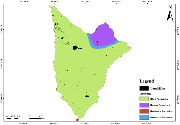
The factor maps used in the susceptibility modelling are shown in Figures 4–13.
Figure 4. Geological map of the study area.
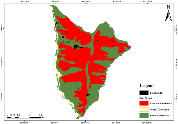
Figure 5. Soil type map of the study area.
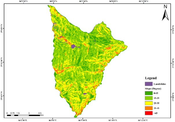
Figure 6. Slope map of the study area.
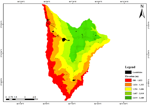
Figure 7. Elevation map of the study area.
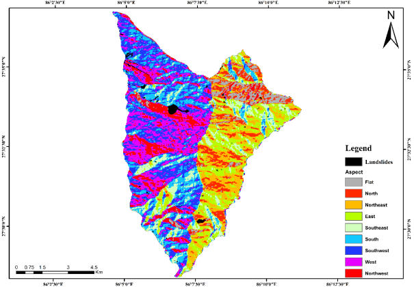
Figure 8. Aspect map of the study area.
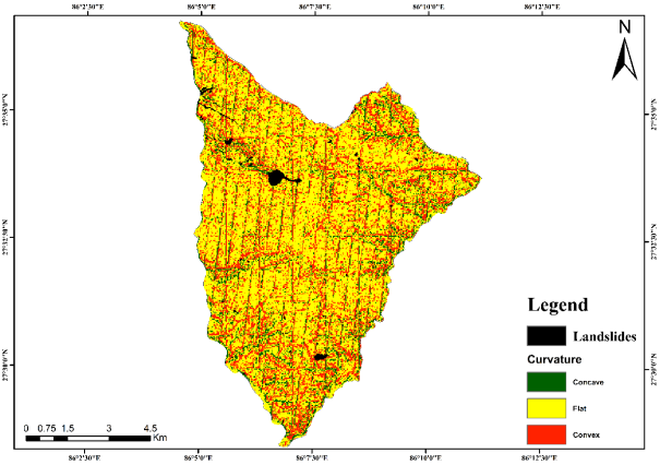
Figure 9. Curvature map of the study area.
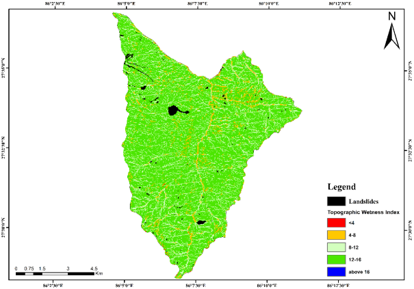
Figure 10. Topographic Wetness Index map of the study area.
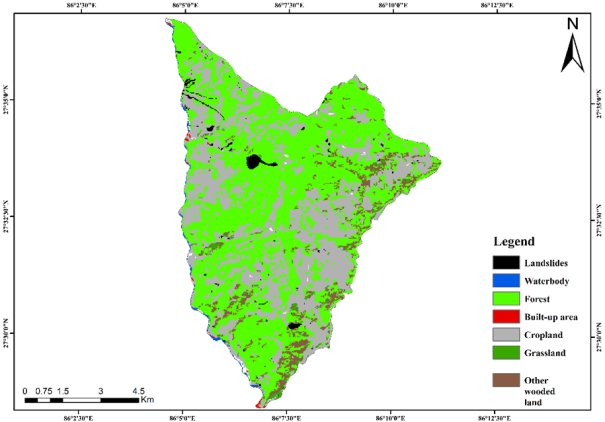
Figure 11. Land use and land cover map of the study area.
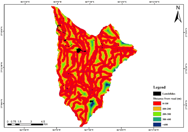
Figure 12. Distance from road map of the study area.
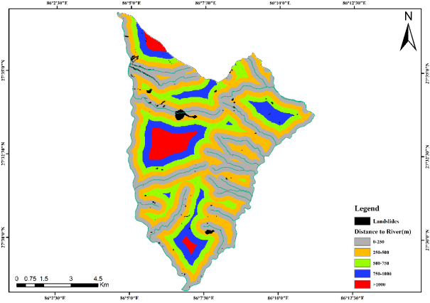
Figure 13. Distance from river map of the study area.
2.6. Preparation and Classification of Conditioning Factors
All conditioning factors were prepared in a raster-based GIS environment using the same projection, spatial extent, cell size and raster alignment. Slope, aspect, curvature, elevation and TWI were derived from the DEM. Distance rasters were generated from the road and river networks using Euclidean distance analysis. Geology, soil type and land use/land cover were converted into categorical raster layers. Continuous variables were divided into classes based on terrain characteristics and the original classification used in the analysis. Categorical variables retained their thematic classes. Each classified factor layer was overlaid with the training landslide inventory to calculate total class pixels and landslide pixels. These values were used to compute model-specific weights.
The TWI was calculated as:
TWI = ln(As/tan β)(1)
where Aₛ is the specific upslope contributing area per unit contour length, ln is natural logarithm and β is the local slope angle expressed in radians. Higher TWI values represent greater potential for moisture accumulation, whereas lower values generally represent steeper or better-drained terrain . For the mathematical notation used below, i denotes a class within a conditioning factor, j denotes a conditioning factor, mj is the number of classes within factor j, and n is the total number of conditioning factors. In this study, n = 10.
2.7. Frequency Ratio Model
The frequency ratio (FR) model is a bivariate statistical method that measures the spatial association between historical landslides and individual classes of conditioning factors. It assumes that future landslides are more likely to occur under terrain and environmental conditions similar to those associated with previous landslides .
The FR value for class i of factor j was calculated as:
FRij= (Lij/ L) / (Aij/ A)(2)
where FRij is the frequency ratio of class i of factor j, Lij is the number of training-landslide cells within that class, L is the total number of training-landslide cells, Aij is the total number of study-area cells within that class, and A is the total number of valid raster cells in the study area. FRij > 1 indicates a positive association, FRij = 1 indicates an average association, and FRij < 1 indicates a comparatively weak association. Each conditioning-factor raster was reclassified using its calculated class-specific FR values. The FR-based landslide susceptibility index was then calculated using pixel-wise summation:
LSI_FR = Σj=1ⁿ FRij(3)
where LSI_FR is the frequency ratio-based landslide susceptibility index and FRij is the weight of the class occupied by the corresponding raster cell in factor j. Higher LSI_FR values indicate greater relative landslide susceptibility.
2.8. Shannon Entropy Model
The Shannon entropy (SE) model applies information theory to measure the degree of disorder, uncertainty and information content associated with the classes of each conditioning factor . Factors showing greater contrast among class-level associations with landslides provide more information and consequently receive greater weights.
First, the FR values of the classes within each factor were normalized as:
Pij= FRij/ Σi=1mʲFRij(4)
where Pij is the normalized probability of class i within factor j and mj is the number of classes in factor j. For every factor, Σi=1mʲ Pij = 1.
The entropy value of factor j was calculated as:
Ej= −kjΣi=1mʲ[Pijln(Pij)](5)
where Ej is the entropy of factor j and kj is a scaling constant defined as:
kj= 1 / ln(mj)(6)
The scaling constant constrains Ej to the interval from 0 to 1. Where Pij = 0, the term Pij ln(Pij) was treated as 0 according to its limiting value.
The information coefficient or degree of divergence was calculated as:
Ij= 1 − Ej(7)
A factor with a larger Ij value shows greater differentiation among its classes and therefore provides more information regarding landslide occurrence. The normalized weight of factor j was calculated as:
Wj= Ij/ Σj=1ⁿ Ij(8)
where Wj is the normalized Shannon entropy weight and Σj=1ⁿ Wj = 1. The final SE-based landslide susceptibility index was calculated as:
LSI_SE = Σj=1ⁿ (Wj× FRij)(9)
where LSI_SE is the Shannon entropy-based susceptibility index. Higher LSI_SE values indicate greater relative susceptibility.
2.9. Statistical Information Index Model
The statistical information index (SII), also known as the information-value method, estimates the contribution of each factor class by comparing its landslide density with the overall landslide density of the study area .
The SII weight for class i of factor j was calculated as:
Wij= ln[(Lij/ Aij) / (L / A)](10)
where Wij is the information weight of class i of factor j, Lij/Aij is the landslide density within that class, and L/A is the overall landslide density of the study area. Positive values indicate above-average landslide density, negative values indicate below-average density, and values close to 0 indicate density approximately equal to the map average. The SII-based landslide susceptibility index was calculated through pixel-wise summation of the relevant class weights:
LSI_SII = Σj=1ⁿ Wij(11)
where LSI_SII is the statistical information index-based susceptibility index. Higher values indicate stronger combined association with landslide occurrence. When a class contained no training-landslide cell, Lij = 0 and the logarithmic expression was undefined. Following the procedure adopted in the original analysis, such a class was assigned the minimum finite SII weight calculated among the remaining classes of the same conditioning factor. This rule was applied consistently to all zero-landslide classes before raster summation .
2.10. Classification of Susceptibility Maps
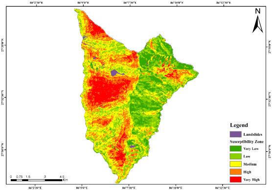
The continuous susceptibility indices generated by FR, SE and SII were independently reclassified into five relative susceptibility classes: very low, low, moderate, high and very high. The Natural Breaks (Jenks) method was used for classification . It identifies break points that minimize within-class variation and maximize between-class variation. Because FR, SE and SII produced different index ranges and distributions, Jenks break values were calculated separately for each model. Therefore, identically named classes across the three models represent relative positions within each model rather than identical numerical thresholds. The resulting maps are presented in Figures 14-16.
2.11. Model Validation Using ROC-AUC
The discriminatory performance of the susceptibility models was evaluated using receiver operating characteristic curves and the area under the ROC curve. The training subset was used to calculate success-rate AUC, whereas the independent validation subset was used to calculate prediction-rate AUC . For threshold-based ROC analysis, landslide cells were treated as positive observations and non-landslide cells used in the ROC procedure were treated as negative observations. At each susceptibility-index threshold, the true-positive rate or sensitivity was calculated as:
TPR = Sensitivity = TP / (TP + FN)(12)
where TP is the number of landslide cells correctly classified above the threshold and FN is the number of landslide cells incorrectly classified below the threshold. The true-negative rate or specificity was calculated as:
TNR = Specificity = TN / (TN + FP)(13)
where TN is the number of non-landslide cells correctly classified below the threshold and FP is the number of non-landslide cells incorrectly classified above the threshold. The false-positive rate was calculated as:
FPR = FP / (FP + TN) = 1 − Specificity(14)
The ROC curve was constructed by plotting TPR against FPR over the range of susceptibility thresholds. Conceptually, the AUC is expressed as:
AUC = ∫₀¹ TPR(u) du(15)
where u represents the false-positive rate. An AUC of 0.5 indicates discrimination equivalent to random ranking, whereas values increasingly above 0.5 indicate progressively better separation. The calculated success AUC values were 0.645 for FR, 0.634 for SE and 0.654 for SII. The corresponding prediction AUC values were 0.623, 0.613 and 0.628. These results indicate modest discriminatory performance, with SII marginally outperforming FR and SE. The ROC curves are presented in Figures 17-19.
2.12. Exposure-Vulnerability Assessment
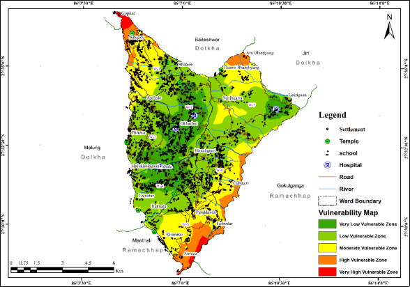
The available datasets represented settlements, population concentration, roads and public-service locations but did not contain detailed household-level social vulnerability, building fragility, income, age, disability or coping-capacity information. The derived layer was therefore interpreted as an exposure-vulnerability index rather than a complete social-vulnerability assessment. Six indicators were included: settlement proximity, population density, hospital proximity, school proximity, road proximity and temple proximity. Distance-based layers were reclassified to a common ordinal scale in which locations closer to mapped settlements and facilities received higher exposure scores. Higher population-density classes also received higher scores. The analytical hierarchy process was used to derive relative indicator weights through pairwise comparison using Saaty’s 1–9 importance scale . The pairwise comparison matrix was represented as A = [akₗ], where akₗ is the relative importance of indicator k compared with indicator l, akk = 1 and aₗk = 1/akₗ. The priority vector was derived from the principal eigenvector:
A v = λmax v(16)
where A is the pairwise comparison matrix, v is its principal eigenvector and λmax is the maximum eigenvalue. The normalized indicator weights were calculated as:
wk= vk/ Σq=1pvq(17)
where wk is the normalized weight of indicator k, p is the number of indicators and Σk=1p wk = 1. Matrix consistency was evaluated using:
CI = (λmax − p) / (p − 1)(18)
CR = CI / RI(19)
where CI is the consistency index and RI is the random consistency index. For six indicators, RI = 1.25 . The calculated CR was 0.0898, below the commonly adopted threshold of 0.10, indicating an adequately consistent comparison matrix.
Table 3. AHP weights for exposure-vulnerability indicators.

Vulnerability indicator

Weight (%)

Interpretation

Settlement proximity

36.03

Direct exposure of people and houses

Population density

26.44

Concentration of exposed population

Hospital proximity

15.58

Access to health service during disaster

School proximity

10.73

Exposure of educational institutions

Road proximity

6.98

Access and road-related exposure

Temple proximity

4.24

Exposure of cultural and social sites

The exposure-vulnerability index was calculated using weighted linear combination:
EV = Σk=1p(wk× xk)(20)
where EV is the exposure-vulnerability index, wk is the normalized AHP weight of indicator k, xk is the reclassified score of that indicator at a raster cell, and p = 6. The resulting continuous EV raster was classified into very low, low, moderate, high and very high classes using the Natural Breaks (Jenks) method. The map is presented in Figure 20.
2.13. Relative Landslide Risk Zonation
The SII susceptibility output was selected for final integration because it produced the highest prediction AUC, although its improvement over FR and SE was small. Because the susceptibility model does not include temporal probability, landslide magnitude or expected loss, the final output should be interpreted as a relative landslide risk map rather than an absolute probabilistic risk map because it integrates landslide susceptibility with exposure-vulnerability indicators and does not explicitly incorporate temporal probability or expected loss . The SII raster was used as a spatial hazard proxy and integrated with the exposure-vulnerability raster.
Before integration, the SII susceptibility index was normalized using min–max scaling:
Sn= (S − Smin) / (Smax− Smin)(21)
where Sn is the normalized susceptibility value, S is the original SII susceptibility value, and Smin and Smax are the minimum and maximum values of the SII raster. The exposure-vulnerability index was similarly normalized as:
EVn= (EV − EVmin) / (EVmax− EVmin)(22)
where EVn is the normalized exposure-vulnerability value, EV is the original index value, and EVmin and EVmax are its minimum and maximum values. Both normalized rasters ranged from 0 to 1. The relative landslide risk index was calculated using a multiplicative model:
Rrel = Sn× EVn(23)
where Rrel is the relative landslide risk index. A high value indicates the spatial coincidence of high susceptibility and high exposure-vulnerability, whereas a low value indicates low susceptibility, low exposure-vulnerability or both. The continuous raster was classified into five classes using Natural Breaks (Jenks). The output represents relative spatial variation within the municipality and should not be interpreted as annual landslide probability, expected casualties or monetary loss. The map is presented in Figure 21.
Google Earth and satellite imagery were used for inventory interpretation. ArcGIS was used for projection, DEM processing, rasterization, resampling, distance analysis, overlay, tabulate-area calculations, raster algebra and map production. Microsoft Excel was used for class-wise statistical calculation, AHP processing and tabulation. Reproducibility was supported by applying a common projection, cell size, spatial extent and alignment to all layers. The same training inventory and class definitions were used when calculating weights for the three models. Intermediate class counts, weights and model outputs should be retained as supplementary data or deposited in a repository when the manuscript is submitted.
3. Results
3.1. Landslide Inventory
A total of 121 landslide locations were identified. The inventory comprised rockfall, debris slide, shallow translational slide, creep and other active or reactivated failures. Field evidence included cracks, seepage, slope bulging, displaced road sections and damage to agricultural land and retaining structures. The training subset contained 85 locations and 938 landslide cells, while the independent validation subset contained 36 locations. Many mapped failures were associated with steep slopes, road cuts, fractured rock, colluvial deposits, river valleys and poorly managed drainage. Representative field-verified examples included the Majhi Gau rockfall and landslide, Tallo Majhi Gau landslide, Narayani Ma. Bhi. instability and Yekle Bari creep.
3.2. Relationship Between Landslides and Conditioning Factors
Slope displayed a positive association with landslide occurrence, and the class above 45° had a high FR value. Landslides were concentrated within the mid-elevation interval of approximately 1351–1680 m, where steep terrain, cultivated slopes, settlements and roads commonly overlap. Aspect influenced distribution, although failures occurred across several orientations. Concave and planar terrain contained comparatively high landslide concentrations, consistent with runoff and moisture convergence in concave positions. River proximity showed a clear relationship: many landslides occurred within 250 m of a river, reflecting toe erosion and valley-side undercutting. Road proximity was similarly important, with many failures located within 100 m of roads, indicating the effects of excavation, steepened cut slopes and altered drainage. Grassland showed a high class-level association in the FR analysis, while forest and cultivated land contained many mapped landslides because of their broad spatial extent and overlap with steep terrain. TWI displayed a variable relationship, indicating that moisture accumulation must be interpreted together with slope, soil and drainage conditions.
3.3. Landslide Susceptibility Maps
All three models produced five susceptibility classes. The FR model classified the largest area as moderate susceptibility. The SE model produced a broader distribution of high and very high classes, whereas SII produced more spatially focused high-susceptibility zones. The three outputs are presented in Figures 14-16.
Figure 14. Landslide susceptibility map produced using the frequency ratio model.
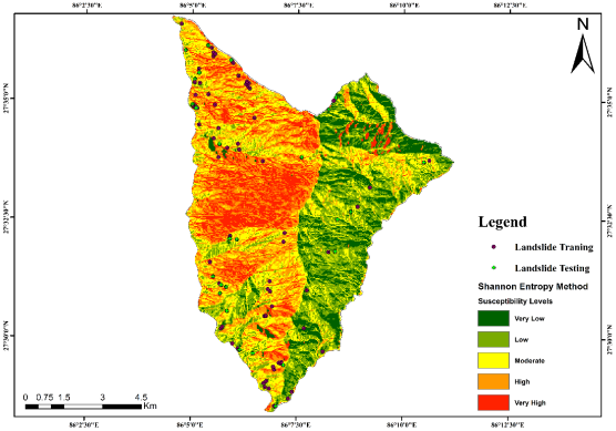
Figure 15. Landslide susceptibility map produced using the Shannon entropy model.
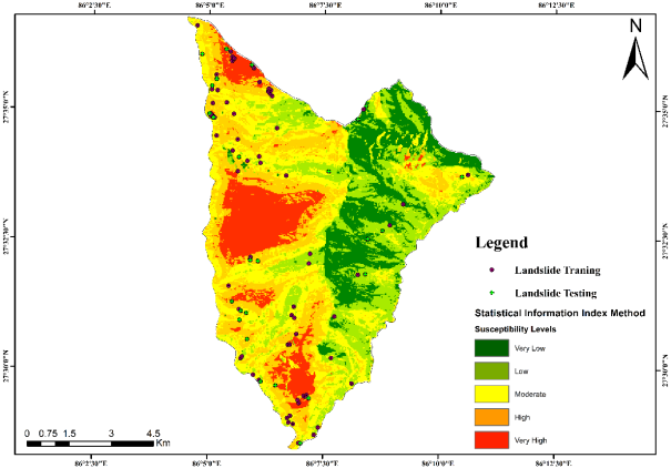
Figure 16. Landslide susceptibility map produced using the statistical information index model.
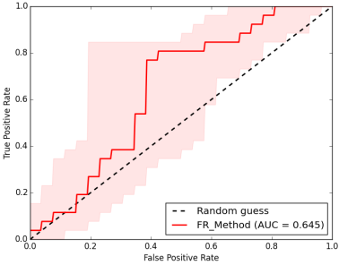
Table 4. Susceptibility-class area distribution.

Susceptibility class

FR area (%)

SE area (%)

SII area (%)

Very low

5.71

7.49

5.02

Low

26.40

10.74

15.37

Moderate

40.99

27.00

50.05

High

22.17

36.35

27.29

Very high

4.73

18.42

2.27

High and very high susceptibility together accounted for 26.90% in FR, 54.77% in SE and 29.56% in SII. The SE model therefore generated the most precautionary spatial classification, while SII concentrated its highest classes into smaller areas.
3.4. Model Validation
SII produced the highest success and prediction AUC values, followed by FR and SE. The differences among prediction AUC values were small: SII exceeded FR by 0.005 and SE by 0.015. SII therefore marginally outperformed the other models rather than demonstrating substantially superior predictive capability. The ROC curves are presented in Figures 17-19.
Table 5. ROC-AUC validation results.

Model

Success AUC

Prediction AUC

Performance interpretation

Frequency ratio

0.645

0.623

Modest discrimination

Shannon entropy

0.634

0.613

Modest discrimination

Statistical information index

0.654

0.628

Highest, but still modest

Figure 17. ROC-AUC curve of the frequency ratio model.
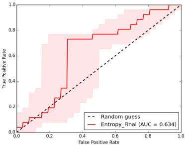
Figure 18. ROC-AUC curve of the Shannon entropy model.
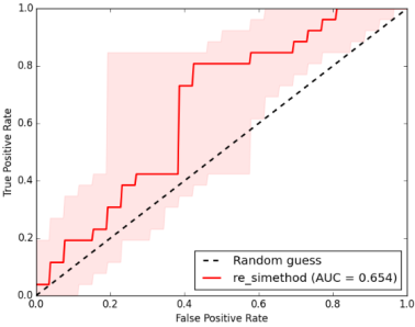
Figure 19. ROC-AUC curve of the statistical information index model.
3.5. Exposure–Vulnerability Pattern
Settlement proximity received the highest AHP weight, followed by population density, hospital proximity, school proximity, road proximity and temple proximity. The CR of 0.0898 indicated an internally consistent comparison matrix. High and very high exposure-vulnerability zones were concentrated around Atmara, Sungure, Dumsi Bhanjhyang, Gahateri and Gobintar. Kiranetar, Gairigaun, Bhatere and parts of the central municipality were mainly within moderate or low classes. Northern and extreme southern areas generally had low to very low index values. The spatial pattern is shown in Figure 20.
Figure 20. AHP-based exposure-vulnerability index for Tamakoshi Rural Municipality.
3.6. Relative Risk Zonation
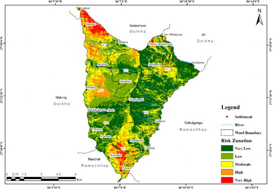
The relative risk map identifies locations where high SII susceptibility overlaps with high exposure-vulnerability. High and very high classes were concentrated mainly in the southern and north-western parts of wards 1, 3 and 5, including areas near Sungure, Archale, Biruwa, Atmara and Kiranetar. Moderate classes surrounded many of the higher-risk zones and represented transitional terrain. Low and very low classes were concentrated mainly in north-eastern, south-western and central parts of wards 4, 6 and 7, including Lamatar, Raamata, Gahateri, Himalpani, Sajhgaira and Gairigaon. The final map is presented in Figure 21.
Figure 21. Relative landslide risk zonation derived from normalized SII susceptibility and exposure-vulnerability indices.

Table 6. Relative risk-class distribution.

Risk class

Approximate area coverage (%)

Main spatial occurrence

High to very high

15

Wards 1, 3 and 5, especially near Sungure, Archale, Biruwa, Atmara and Kiranetar

Moderate

21

Transitional areas surrounding high-risk zones

Low to very low

63

Mainly wards 4, 6 and 7 and relatively stable central, north-eastern and south-western areas

Note: Percentages are rounded and therefore do not sum exactly to 100.
4. Discussion
4.1. Controls of Landslide Occurrence
The results show that landslide occurrence in Tamakoshi Rural Municipality is mainly controlled by the combined influence of of slope, elevation, aspect, curvature, lithology, land use, river proximity, road proximity and local hydrological conditions. The concentration of landslides on moderate to steep slopes confirms the importance of terrain steepness in slope instability. Although the slope class above 45° showed a strong class-level association, most landslide pixels were recorded in the 25°–35° class because this class covers a larger portion of the study area and commonly overlaps with roads, agricultural land and settlements. This indicates that slope does not act alone; landslide occurrence is the result of interaction among terrain condition, material property, drainage and human disturbance .
Elevation also influenced landslide distribution. The highest concentration of landslides occurred within the 1351–1680 m elevation range, where weathered slopes, agricultural terraces, road sections and settlement areas commonly overlap. Aspect showed higher landslide concentration on south, southwest, west and northwest-facing slopes. This pattern may be related to rainfall exposure, solar radiation, moisture variation and weathering intensity. Similarly, curvature influenced landslide occurrence because concave and planar slopes can support runoff concentration, water retention and translational movement.
River proximity showed a clear relationship with landslide occurrence. Many landslides were concentrated within 250 m of rivers and streams, indicating the role of toe erosion, bank cutting and slope undercutting. Road proximity was also important, with many landslides located within 100 m of road corridors. Road construction in hilly terrain often disturbs natural slope geometry, removes toe support and changes drainage pathways, thereby increasing the likelihood of slope failure during rainfall events.
The land use and land cover result should be interpreted together with slope and geology. Forest and cultivated land contained many landslides because they cover large parts of the municipality and often occur on steep terrain. Although vegetation generally helps stabilize shallow soil, forest cover may not prevent failures where slopes are controlled by fractured rock, deep weathering, river erosion or poor drainage. Cultivated terraces may also become unstable where drainage is not properly managed.
4.2. Comparison of FR, SE and SII Models
The three susceptibility models produced different spatial patterns because they use different weighting procedures. The Frequency Ratio (FR) model is simple and directly represents the relationship between landslide occurrence and each conditioning-factor class. Because of its transparency and ease of interpretation, the FR model has been widely applied and compared with other statistical and machine-learning approaches in landslide susceptibility studies . The Shannon Entropy (SE) model produced the largest high and very high susceptibility area, indicating a more precautionary classification. The Statistical Information Index (SII) model produced the highest AUC values and a more focused distribution of high-susceptibility zones. SII assigns both positive and negative information values, which helps distinguish classes with above-average and below-average landslide density . The validation results showed that SII performed slightly better than FR and SE. The success and prediction AUC values were 0.654 and 0.628 for SII, 0.645 and 0.623 for FR, and 0.634 and 0.613 for SE, respectively. However, the differences among the three models were small. Therefore, SII can be considered the most suitable model for this study area, but not overwhelmingly superior. The modest AUC values indicate that landslide occurrence in the study area is controlled by complex local conditions that are not fully captured by bivariate statistical models.
The results are consistent with previous landslide susceptibility studies in Nepal and similar Himalayan terrain, which show that bivariate statistical models can provide useful susceptibility maps in data-limited areas . However, the relative performance of each model varies from place to place depending on landslide inventory quality, conditioning-factor selection, factor classification, spatial resolution and geomorphic setting. This confirms the need for site-specific model comparison before selecting a final susceptibility map.
4.3. Relative Risk Zonation and Planning Implications
The relative risk zonation prepared in this study provides useful information for local planning and disaster risk reduction. High and very high-risk zones cover about 15% of the municipality and are mainly concentrated in wards 1, 3 and 5, particularly around Sungure, Archale, Biruwa, Atmara and Kiranetar. These areas should be prioritized for detailed field investigation, slope monitoring, road drainage improvement and landslide mitigation planning. Moderate-risk zones should also be considered carefully during infrastructure development because future road expansion or drainage alteration may increase instability. Low and very low risk zones are relatively more stable within the municipal context, especially in parts of wards 4, 6 and 7. However, these areas should not be considered completely free from landslide hazard. The generated map should be used as a regional planning and prioritization tool rather than a replacement for detailed geotechnical investigation before construction.
4.4. Limitations
The study has some limitations. The landslide inventory may not include all old, small or vegetation-covered landslides. The use of 30 m resolution datasets may limit the detection of small slope failures and narrow road-cut landslides. Rainfall intensity, antecedent moisture, soil depth and detailed geotechnical parameters were not included due to data limitations. Similarly, the vulnerability assessment was based on available exposure indicators and did not include detailed household-level socio-economic vulnerability. Therefore, the final output should be interpreted as a relative landslide risk zonation map rather than an absolute probabilistic risk map. Despite these limitations, the study provides a transparent and reproducible GIS-based approach for comparing FR, SE and SII models and integrating susceptibility with exposure-vulnerability information. The results can support municipal-level land-use planning, road management, field prioritization and disaster risk reduction in Tamakoshi Rural Municipality.
5. Conclusion
This study compared Frequency Ratio (FR), Shannon Entropy (SE) and Statistical Information Index (SII) models for landslide susceptibility assessment and relative risk zonation in Tamakoshi Rural Municipality, Dolakha, Nepal. A total of 121 landslide locations were mapped using Google Earth imagery, satellite-image interpretation and field verification. Ten conditioning factors were used in the analysis: slope, aspect, curvature, elevation, Topographic Wetness Index (TWI), lithology, soil type, land use/land cover, distance from roads and distance from rivers. The results showed that landslides are mainly associated with steep to moderately steep slopes, mid-elevation terrain, proximity to rivers and proximity to roads. River undercutting, road excavation, poor drainage, fractured lithology and human disturbance were identified as important contributors to slope instability. Among the three models, SII produced the highest success and prediction AUC values of 0.654 and 0.628, followed by FR with 0.645 and 0.623 and SE with 0.634 and 0.613. Although SII performed slightly better, all three models showed modest predictive performance, indicating the complex nature of landslide occurrence in the study area.
The exposure-vulnerability assessment showed that settlement proximity and population density were the most influential indicators. By integrating the SII-based susceptibility output with the exposure-vulnerability index, the relative risk map identified about 15% of the municipality as high to very high risk, mainly in wards 1, 3 and 5. Moderate risk zones covered about 21%, while low to very low risk zones covered about 63% of the municipality. The study provides a practical and reproducible GIS-based approach for landslide susceptibility and relative risk assessment in data-limited mountainous regions. The resulting maps can support field prioritization, road and drainage management, land-use planning and local disaster risk reduction. However, the maps should be used as regional planning tools and supplemented by detailed site-specific geological and geotechnical investigation before major infrastructure development or relocation decisions.
Abbreviations

AHP

Analytical Hierarchy Process

AUC

Area Under the Curve

DEM

Digital Elevation Model

EV

Exposure-Vulnerability

FR

Frequency Ratio

GIS

Geographic Information System

LSI

Landslide Susceptibility Index

LSM

Landslide Susceptibility Mapping

LULC

Land Use/Land Cover

ROC

Receiver Operating Characteristic

SE

Shannon Entropy

SII

Statistical Information Index

TWI

Topographic Wetness Index

UTM

Universal Transverse Mercator

WGS

World Geodetic System

Author Contributions
Nabaraj Bajagain: Conceptualization, Data curation, Formal Analysis, Investigation, Methodology, Project administration, Software, Visualization, Writing – original draft
Bhuwan Singh Bisht: Conceptualization, Methodology, Project administration, Supervision, Resources, Validation, Writing – review & editing
Conflicts of Interest
The authors declare no conflicts of interest.
References
[1] Ado M, Amitab K, Maji AK, Jasińska E, Gono R, Leonowicz Z, Jasiński M (2022) Landslide susceptibility mapping using machine learning: A literature survey. Remote Sensing 14(13): 3029.
[2] Ale Magar T, Bhandari BP (2025) Application of the bivariate frequency ratio method for landslide susceptibility mapping of Manthali Municipality, Ramechhap District, Nepal. Nepal Journal of Environmental Science 13(1): 43–60.
[3] Ayer PB, Bhandari BP (2024) Landslide susceptibility mapping using frequency ratio and weight of evidence models in Purchaudi Municipality, Baitadi District, Nepal. Nepal Journal of Environmental Science 12(2): 59–72.
[4] Beven KJ, Kirkby MJ (1979) A physically based, variable contributing area model of basin hydrology. Hydrological Sciences Bulletin 24(1): 43–69.
[5] Bhandari BP, Dhakal S, Tsou CY (2024) Assessing the prediction accuracy of frequency ratio, weight of evidence, Shannon entropy, and information value methods for landslide susceptibility in the Siwalik Hills of Nepal. Sustainability 16(5): 2092.
[6] Chung CJF, Fabbri AG (2003) Validation of spatial prediction models for landslide hazard mapping. Natural Hazards 30(3): 451–472.
[7] Dahal RK, Hasegawa S (2008) Representative rainfall thresholds for landslides in the Nepal Himalaya. Geomorphology 100(3–4): 429–443.
[8] Dahal RK, Hasegawa S, Masuda T, Yamanaka M (2006) Roadside slope failures in Nepal during torrential rainfall and their mitigation. In: Disaster mitigation of debris flows, slope failures and landslides. Universal Academy Press, Tokyo, pp 503–514.
[9] Dhital MR (2015) Geology of the Nepal Himalaya: Regional perspective of the classic collided orogen. Springer, Cham, 498 pp.
[10] Ercanoglu M, Gokceoglu C (2002) Assessment of landslide susceptibility for a landslide-prone area, north of Yenice, NW Turkey, by fuzzy approach. Environmental Geology 41: 720–730.
[11] Fell R, Corominas J, Bonnard C, Cascini L, Leroi E, Savage WZ (2008) Guidelines for landslide susceptibility, hazard and risk zoning for land-use planning. Engineering Geology 102(3–4): 85–98.
[12] Guzzetti F, Carrara A, Cardinali M, Reichenbach P (1999) Landslide hazard evaluation: A review of current techniques and their application in a multi-scale study, central Italy. Geomorphology 31(1–4): 181–216.
[13] Jenks GF (1967) The data model concept in statistical mapping. International Yearbook of Cartography 7: 186–190.
[14] Lee S, Talib JA (2005) Probabilistic landslide susceptibility and factor effect analysis. Environmental Geology 47: 982–990.
[15] Ministry of Home Affairs (2019) Nepal Disaster Report 2019. Government of Nepal, Kathmandu.
[16] Pathak D (2016) Knowledge-based landslide susceptibility mapping in the Himalayas. Geoenvironmental Disasters 3: 8.
[17] Pourghasemi HR, Mohammady M, Pradhan B (2012) Landslide susceptibility mapping using index of entropy and conditional probability models in GIS: Safarood Basin, Iran. Catena 97: 71–84.
[18] Regmi AD, Devkota KC, Yoshida K, Pradhan B, Pourghasemi HR, Kumamoto T, Akgun A (2014) Application of frequency ratio, statistical index, and weights-of-evidence models and their comparison in landslide susceptibility mapping in Central Nepal Himalaya. Arabian Journal of Geosciences 7(2): 725–742.
[19] Reichenbach P, Rossi M, Malamud BD, Mihir M, Guzzetti F (2018) A review of statistically based landslide susceptibility models. Earth-Science Reviews 180: 60–91.
[20] Roodposhti MS, Aryal J, Shahabi H, Safarrad T (2016) Fuzzy Shannon entropy: A hybrid GIS-based landslide susceptibility mapping method. Entropy 18(10): 343.
[21] Saaty TL (1977) A scaling method for priorities in hierarchical structures. Journal of Mathematical Psychology 15(3): 234–281.
[22] Saaty TL (1980) The analytic hierarchy process: Planning, priority setting, resource allocation. McGraw-Hill, New York, 287 pp.
[23] Saha AK, Gupta RP, Sarkar I, Arora MK, Csaplovics E (2005) An approach for GIS-based statistical landslide susceptibility zonation with a case study in the Himalayas. Landslides 2: 61–69.
[24] Saud TB, Ayer PB, Awasthi MP, Bhandari BP, Joshi NR (2025) Application of bivariate frequency ratio and information value models for landslide susceptibility in Thuligad watershed of far-western Nepal. Discover Geoscience 3: 193.
[25] Shannon CE (1948) A mathematical theory of communication. Bell System Technical Journal 27(3): 379–423.
[26] Soeters R, van Westen CJ (1996) Slope instability recognition, analysis and zonation. In: Turner AK, Schuster RL (Eds) Landslides: Investigation and mitigation. Transportation Research Board Special Report 247. National Academy Press, Washington DC, pp 129–177.
[27] Upreti BN, Dhital MR (1996) Landslide studies and management in Nepal. International Centre for Integrated Mountain Development, Kathmandu, 87 pp.
[28] van Westen CJ (1997) Statistical landslide hazard analysis. ILWIS 2: 73–84.
[29] van Westen CJ, Castellanos E, Kuriakose SL (2008) Spatial data for landslide susceptibility, hazard, and vulnerability assessment: An overview. Engineering Geology 102(3–4): 112–131.
[30] Yilmaz I (2009) Landslide susceptibility mapping using frequency ratio, logistic regression, artificial neural networks and their comparison: A case study from Kat landslides, Tokat, Turkey. Computers and Geosciences 35(6): 1125–1138.
Cite This Article
  • APA Style

    Bajagain, N., Bisht, B. S. (2026). Comparative GIS-Based Landslide Susceptibility and Relative Risk Assessment Using Frequency Ratio, Shannon Entropy and Statistical Information Index Models. American Journal of Applied Scientific Research, 12(3), 81-102. https://doi.org/10.11648/j.ajasr.20261203.13

    Copy | Download

    ACS Style

    Bajagain, N.; Bisht, B. S. Comparative GIS-Based Landslide Susceptibility and Relative Risk Assessment Using Frequency Ratio, Shannon Entropy and Statistical Information Index Models. Am. J. Appl. Sci. Res. 2026, 12(3), 81-102. doi: 10.11648/j.ajasr.20261203.13

    Copy | Download

    AMA Style

    Bajagain N, Bisht BS. Comparative GIS-Based Landslide Susceptibility and Relative Risk Assessment Using Frequency Ratio, Shannon Entropy and Statistical Information Index Models. Am J Appl Sci Res. 2026;12(3):81-102. doi: 10.11648/j.ajasr.20261203.13

    Copy | Download

  • @article{10.11648/j.ajasr.20261203.13,
      author = {Nabaraj Bajagain and Bhuwan Singh Bisht},
      title = {Comparative GIS-Based Landslide Susceptibility and Relative Risk Assessment Using Frequency Ratio, Shannon Entropy and Statistical Information Index Models},
      journal = {American Journal of Applied Scientific Research},
      volume = {12},
      number = {3},
      pages = {81-102},
      doi = {10.11648/j.ajasr.20261203.13},
      url = {https://doi.org/10.11648/j.ajasr.20261203.13},
      eprint = {https://article.sciencepublishinggroup.com/pdf/10.11648.j.ajasr.20261203.13},
      abstract = {Landslides are recurrent geomorphic hazards in the Nepal Himalaya, where fragile geology, steep terrain, monsoonal rainfall and expanding road construction increase slope instability. This study assesses landslide susceptibility and relative risk in Tamakoshi Rural Municipality, Dolakha, Nepal, by comparing three GIS-based bivariate models: frequency ratio (FR), Shannon entropy (SE) and statistical information index (SII). A landslide inventory of 121 events was prepared from Google Earth imagery, satellite-image interpretation and field verification, and divided into 70% training and 30% validation subsets. Ten conditioning factors were analysed at 30 m spatial resolution: slope, aspect, curvature, elevation, topographic wetness index, lithology, soil type, land use/land cover, distance from roads and distance from rivers. Model discrimination was evaluated using receiver operating characteristic-area under the curve analysis. Landslides were concentrated on steep, mid-elevation slopes, particularly within 250 m of rivers and 100 m of roads, indicating the influence of fluvial undercutting, road excavation and drainage disturbance. SII produced the highest success and prediction AUC values (0.654 and 0.628), followed by FR (0.645 and 0.623) and SE (0.634 and 0.613), although all three models showed only modest discrimination. An AHP-based exposure–vulnerability index was prepared from settlement, population, road, school, hospital and temple indicators. The resulting relative risk zonation identified approximately 15% of the municipality as high or very high risk, mainly in wards 1, 3 and 5. The findings provide a spatial basis for field prioritization, risk-sensitive land-use planning and local disaster risk reduction.},
     year = {2026}
    }
    

    Copy | Download

  • TY  - JOUR
    T1  - Comparative GIS-Based Landslide Susceptibility and Relative Risk Assessment Using Frequency Ratio, Shannon Entropy and Statistical Information Index Models
    AU  - Nabaraj Bajagain
    AU  - Bhuwan Singh Bisht
    Y1  - 2026/07/24
    PY  - 2026
    N1  - https://doi.org/10.11648/j.ajasr.20261203.13
    DO  - 10.11648/j.ajasr.20261203.13
    T2  - American Journal of Applied Scientific Research
    JF  - American Journal of Applied Scientific Research
    JO  - American Journal of Applied Scientific Research
    SP  - 81
    EP  - 102
    PB  - Science Publishing Group
    SN  - 2471-9730
    UR  - https://doi.org/10.11648/j.ajasr.20261203.13
    AB  - Landslides are recurrent geomorphic hazards in the Nepal Himalaya, where fragile geology, steep terrain, monsoonal rainfall and expanding road construction increase slope instability. This study assesses landslide susceptibility and relative risk in Tamakoshi Rural Municipality, Dolakha, Nepal, by comparing three GIS-based bivariate models: frequency ratio (FR), Shannon entropy (SE) and statistical information index (SII). A landslide inventory of 121 events was prepared from Google Earth imagery, satellite-image interpretation and field verification, and divided into 70% training and 30% validation subsets. Ten conditioning factors were analysed at 30 m spatial resolution: slope, aspect, curvature, elevation, topographic wetness index, lithology, soil type, land use/land cover, distance from roads and distance from rivers. Model discrimination was evaluated using receiver operating characteristic-area under the curve analysis. Landslides were concentrated on steep, mid-elevation slopes, particularly within 250 m of rivers and 100 m of roads, indicating the influence of fluvial undercutting, road excavation and drainage disturbance. SII produced the highest success and prediction AUC values (0.654 and 0.628), followed by FR (0.645 and 0.623) and SE (0.634 and 0.613), although all three models showed only modest discrimination. An AHP-based exposure–vulnerability index was prepared from settlement, population, road, school, hospital and temple indicators. The resulting relative risk zonation identified approximately 15% of the municipality as high or very high risk, mainly in wards 1, 3 and 5. The findings provide a spatial basis for field prioritization, risk-sensitive land-use planning and local disaster risk reduction.
    VL  - 12
    IS  - 3
    ER  - 

    Copy | Download

Author Information
  • Abstract
  • Keywords
  • Document Sections

    1. 1. Introduction
    2. 2. Materials and Methods
    3. 3. Results
    4. 4. Discussion
    5. 5. Conclusion
    Show Full Outline
  • Abbreviations
  • Author Contributions
  • Conflicts of Interest
  • References
  • Cite This Article
  • Author Information