In asset pricing applications one of the most powerful and widely used models is the famous Black-Sholes model. In applications of stock option pricing, the resulting Black-Scholes formula requires inputting several values, including the current price of the stock and the market volatility. The question of how to input the volatility in real-time can be very challenging, as commonly utilized measures, such as the volatility index (VIX), can be viewed as lagging economic indicators. This research discusses a scheme that applies a mathematical model which defines how far the current market value is above or below from where macroeconomic conditions would expect it to be. In prior research, a regression model was created to define a framework that theoretically outlined a new measure related to market volatility. When computing various financial predictions, such as evaluating the fair price of an option, this measure can be used to supplement common current measures, such as the VIX. In the current work, several mathematical methods, including machine learning, are investigated to determine if improvements to accuracy can be made, and define a practically usable scheme. Slight improvements to accuracy were discovered in comparison to the prior regression model; the Principal Component Analysis method is recommended for usage in real time applications.
This is an Open Access article, distributed under the terms of the Creative Commons Attribution 4.0 International License (http://creativecommons.org/licenses/by/4.0/), which permits unrestricted use, distribution and reproduction in any medium or format, provided the original work is properly cited.
The prediction of the stock market valuation is a very complex problem that poses significant challenges to mathematical modelling; however, it is known that models, such as the famous Black Scholes Stochastic Partial Differential Equation
[1]
Black, F., Scholes, M. The Pricing of Options and Corporate Liabilities, Journal of Political Economy. 1973, 81(3), 637-654.
can be used to find the fair price of options for individual stocks over longer time domains. For example, given a stock which has the price today as x0, the Black Scholes Formula will give the fair price of the option to be
Here, the call option maturity date is defined by T, the strike price is defined by k, the risk free interest rate is defined by r, and N(X) is the cumulative standard normal distribution. In this work, we investigate the value of σ, the “volatility.” What value to use for volatility has been debated for many years, dating back to the pioneering work Fisher Black and Merton Scholes, who themselves made some comments
[1]
Black, F., Scholes, M. The Pricing of Options and Corporate Liabilities, Journal of Political Economy. 1973, 81(3), 637-654.
about σ. A common understanding is that σ2 can be defined as the variance of the asset under consideration. However, it is not so obvious as to how one can obtain that value in real world applications in real time. If one is utilizing yesterday’s data, the stock has already moved and the trader may have missed their buying or selling opportunity When applying this logic to the border market, e.g. using the S&P 500 as a benchmark, experts in the financial management domain often look to the Chicago Board Options Exchange Volatility Index (VIX) index
[4]
Whaley, R. The Investor Fear Gauge. The Journal of Portfolio Management, 2000. 26(3), 12-17.
In this work we seek to update a mathematical model that could be used to define a predictive measure of volatility for the broad market. This measure is essentially defined as how far the current value of the market is off from the value that current macroeconomic measures expect that valuation to be. It is hypothesized that the results of such a model can be used to create a value of σ that is more of a forward looking, or at least real time, volatility as opposed to a lagging economic indicator. For practical application, this measure could be used alongside the readily available and useful data of the VIX index. For example, when computing the Black Scholes Formula the value of σ inputted could be an average of this new measure and the VIX, or some sort of “regime switching” machine learning scheme could be applied where this new measure’s weight in a weighted average would be increased during certain periods of time.
In our original studies
[6]
Smith, T., Subasi, E. Rattansi, A. A Regression Model to improve the performance of Black-Scholes using macroeconomic predictors. International Journal of Mathematics Trends and Technology. 2014, 5(2), 108-111.
[7]
Smith, T., Hawkins, A. An Economic Regression Model to Predict Market Movements. International Journal of Mathematics Trends and Technology. 2015, 28(1), 1-3.
, a four variable regression model was used on a fixed data set to define the general concept. Also, a scheme was defined, and it was verified that this measure performed better than using the VIX by analysing its performance on several historical data sets. In the current work the idea is extended to experiment with a higher dimensional data set and more modern models, including several machine learning models.
The original intent of these works was to study the volatility problem, but an interesting side note result worthy of mentioning is the practical application of the model’s direct application. Namely, using real time macroeconomic predictors to identify times when the overall market is severely overvalued or undervalued. For example, at the time of this writing the S&P 500 is up just shy of 17% year-to-date and has averaged annual gains of approximately 16% over the past five years. This may lead one to believe the market is extremely overvalued; however, such direct comparisons can be misleading as a return during a time period of high inflation, and resulting reduction in currency purchasing power, is different than the same return in a low-inflation environment. Our model explicitly adjusts for these macroeconomic factors, enabling a more precise mathematical characterization of overvalued and undervalued market states.
2. Methods & Summary of Prior Models
In prior research, the four predictor variables utilized to build the model were: the consumer price index (CPI), the producer price index (PPI), gross domestic product (GDP), along with the money supply (M). The original human choice of these predictors - the feature engineering process - was based on a method previously used at an investment firm
[8]
Park, S. Reducing the Noise in Forecasting. Wentworth. New York City 2005.
[8]
. The prior work manually created a regression model using monthly data from January 1990 to July 2013. This original model worked well, its coefficient of determination was approximately 0.8. A numerical scheme was constructed to define the alternate measure of volatility as previously described. A comparison was done using the value of the VIX for σ, versus using our method, and it was showed increased performance in comparison to the Black Scholes using VIX during several historical data sets, including one that contained the 2008 time period. Hence, suggesting that the approach has practical merit.
As the availability of data had grown rapidly in the preceding years, it was decided to revisit the study. Various other predictor variables were added into the design of the model. In that work
[7]
Smith, T., Hawkins, A. An Economic Regression Model to Predict Market Movements. International Journal of Mathematics Trends and Technology. 2015, 28(1), 1-3.
, the added variables were: national unemployment rate, government interest rate, value of international stock markets, value of exchange rates of various international currencies, along with various consumer confidence polls. This process was done following classical regression model building analysis, and the best performing model was the one using the four predictor variables: GDP, FFR, M, and the unemployment rate. However, from a statistical analysis point of view one should use a three-variable model without the fed fund rate (FFR) as, surprisingly, that predictor variable did not have a significant test statistic, its test stat was just -0.84. Therefore, the final model utilized was
(1)
Here, Z1 is representing the GDP data variable, Z2 is the M data variable and Z3 is the U data variable, along with the Y variable representing the value of the SP 500 at the corresponding time. The Z label is utilized for our predictors as the data was normalized prior to running models. The model yielded the following results.
Table 1. Prior model’s statistical summary.
Coefficients
Standard Error
t Stat
Intercept
965.0635
6.659789
144.909
GDP
362.1807
28.36177
12.77003
MS
183.392
28.53035
6.427962
UI
-173.762
7.021221
-24.7482
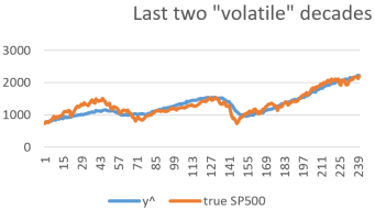
Along with a solid F statistic of two thousand three hundred and thirty. In a commonsense approach, as one can see in the graph below, that this model predicted “market top before market crash,” with large values of our measure during the time period leading upto 2008.
The information within Figure 2 could be very useful for traders to predict long term market buy/sell points; however, the interest of this research is to use the model to predict an alternate measure of volatility. In the prior study,
[9]
Smith, T., Rajan, A. A Regression Model to Predict Stock Market Mega Movements and/or Volatility using both Macroeconomic indicators & Fed Bank Variables. International Journal of Mathematics Trends and Technology. 2017, 49(3), 165-167.
a scheme was created, along with its corresponding Matlab code, to define this new measure of volatility. In that work, results were developed that showed it performed better that the VIX. For illustration, if one were to define the deviation of this model output y^ from the true SP500 value as Δy, the volatility 𝞼 can be defined in a pricewise manner, such as
(2)
3. Results & Analysis of New Learning Models
So far, all the mathematics conducted have been using classical statistical models, namely regression with a multivariable predictor. In the following we investigate if the accuracy can be improved by applying various modern machine learning methods on a larger data set. In theory, this method could be applied to a much larger data set which could consists of any measurements that are available monthly and the researcher believes they could have the ability to increase the prediction power. Then a deep learning process of feature engineering could be applied; however, for our current work we limited the data to a selection of just 12 features that were both readily available from trusted sources and are known to have a strong correlation to the overall economy and/or stock market assets prices. Hence, the work here still falls in the realm of a “human in the loop” feature selection process as a regular machine learning process. The logic here is that while it could be useful to scale out our original model in an attempt to perfect its accuracy, it is essential to remember that computational efficiency is an important consideration in financial applications. A more efficient model that may be slightly less accurate but quicker, is likely to be preferable over a model that is slightly more accurate but very costly to compute. In addition, while advanced learning models may pick up on some patterns within data they are trained on, it is not guaranteed that they truly are predictive of future patterns, especially in such a complex problem of stock market behavior; thus, it is preferred to apply a “human in the loop” feature engineering process where the researcher identifies real predictor variables that have logical connection to the economy. Advanced learning models may be useful for short term movements, such as applications for day traders, but that is not the purpose of our study; our work is grounded in economic theory and the mathematical trust in regression to the mean!
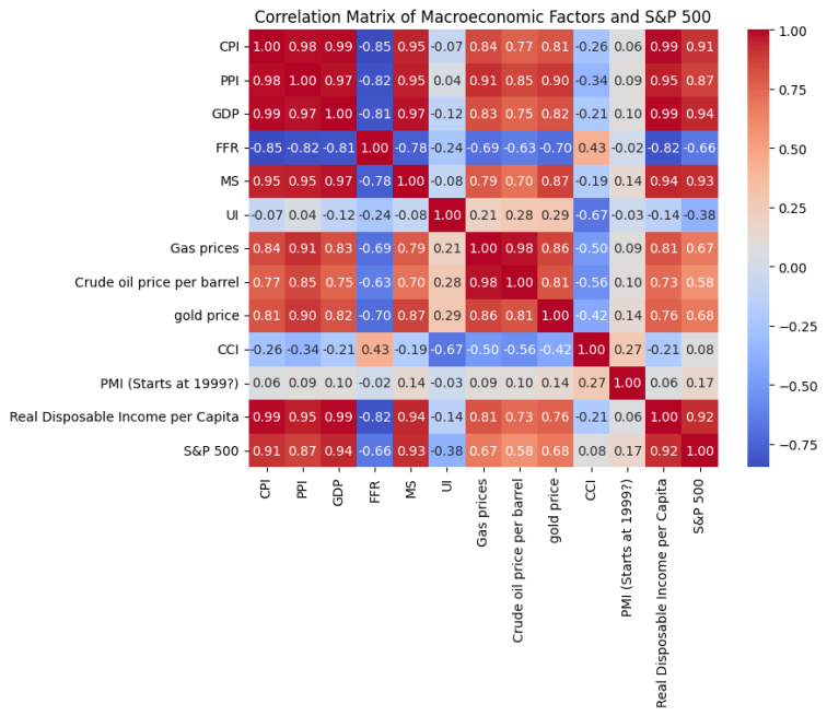
The data used for the research consists of 12 predictor variable columns and 498 rows. The 498 entries contain data for each of the predictor variables, in addition to the response variable of the SP 500, recorded monthly from Jan 1984 to May 2019. The data included the following predictor variables: CPI, PPI, GDP, FFR, M, Unemployment Rate, Consumer Confidence Index (CCI), Price Manager’s Index (PMI), National Average Gas Prices, Crude Oil Price per Barrel, Gold Price and Real Disposable Incomer per Capita.
Prior to running the various machine learning models, a correlation matrix was plotted, with the expected insight being that many of the variables are highly correlated. For example, and as illustrated in the Figure 2 below, the Real Disposable Income has a 99% correlation with both CPI and GDP.
This indicates strong multicollinearity in the dataset, which can cause numerical instability. Due to this, Real Disposable Income was chosen to be removed, as it destabilized the original runs of Linear and Lasson regression. Furthermore, it was logically preferred to keep the CPI and GDP measurements as those are direct measurements from established government resources, while the disposable income measurements often rely on reports from individuals and/or corporations which may not be as accurate. This leaves the final data set with 11 predictor variables.
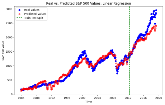
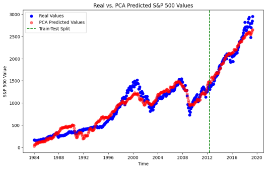
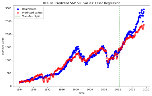
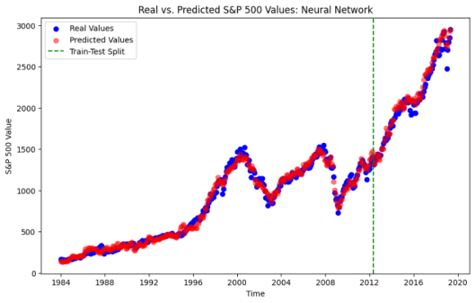
After data cleaning and basic analysis, the data was transformed using the scikit-learn Standard Scaler. Finally, the data was separated into a training and testing set with an 80/20 split temporally, with the split date being May 201. Several models were run as illustrated in the figures below which also contain some high-level performance metrics summaries within their labeling. The corresponding ordering is Linear Regression, PCA then Linear Regression, Lasso, Forward Neural Net.
Figure 6. The Neural Network, R2 on testing data = 96%.
The main takeaways are the following. It is not surprising see that the ordinary least-squares regression fit the training data we, but did not perform well in predictive accuracy; the model consistently predicted values that were lower than the corresponding testing data values. In prior research, it was believed that while the model was showing promise, concerns for its ability to perform on future data were uncertain; hence, the motivation for our current research. It was surprising to see that the Lasso Regression performed poorly and did not provide insight into removable features; this could be a result of the issue of variables withing the data being highly correlated. This was resolved in the Principal Component Analysis method! In the PCA method four principal components were used, capturing just under 93% of the explained variance. This fixed instability and provided improved results. The several other models run, the more popular machine learning models, did technically perform slightly better The tree based methods – Decision Tree, Random Forest and XGBoost – did nor perform well on the dataset, likely due to the persistent upwards trend in the data and it showed an inability to predict on data outside of the training data, which is a common issue with such models. A machine learning model – forward feed neural net – was discovered that did perform slightly better, and it is expected that if other machine learning models were run it is likely that one could be identified that adds additional slight improvement to the accuracy; however, this leads back to the conversation about cost of computing versus slight improvements to accuracy.
4. Discussion
In previous works a regression model was created to define a scheme that can be utilized to define a measure of market volatility that can be used to complement commonly used tools such as volatility index (VIX). The original model had decent performance with its coefficient of determination being approximately 80%. This was later refined to define a three-predictor variable model which had slightly improved performance. In the current work several advanced statistical methods, in addition to machine learning methods, were investigated to determine if improvements can be made. Mathematically, the best preforming model was a machine learning model. The second-best performing model was the PCA which yielded a slightly lower, but similar, coefficient of determination. The latter is more desirable for practical applications due to several reasons. Firstly, while its performance is slightly lowered, it is expected that with the accuracy it is presenting it will be able to identify major trends, and it is a quicker model to train and run. This can be of practical importance for real-time applications as it can be trained through a relatively quick optimization procedure as opposed to the computationally costly process of advanced machine learning needed computations required for the neural network model. Also, the resulting model equation from the PCA is in the format of a well-known regression equation, so it would be expected that in applications it would be more interactable to a wider range of users. Regardless, the improvements when comparing either the PCA or the neural network to the prior method are impressive!
5. Conclusions
The regression after PCA is a classical model that not only has a lower cost of computation, but it also has the benefit of being a user-friendly model that many working professions have some knowledge and/or prior experience working with. The conclusion is that this method would be the most practical for implementation, and addressing. This model would be an improvement over the priors and has the ability to be a very useful tool both for our application of interest, the volatility problem
[10]
Kownatzki, C. How Good is the VIX as a Predictor of Market Risk. Journal of Accounting and Finance, 2016. 16(6), 1-22.
Smith, T., Subasi, E. Rattansi, A. A Regression Model to improve the performance of Black-Scholes using macroeconomic predictors. International Journal of Mathematics Trends and Technology. 2014, 5(2), 108-111.
[7]
Smith, T., Hawkins, A. An Economic Regression Model to Predict Market Movements. International Journal of Mathematics Trends and Technology. 2015, 28(1), 1-3.
Park, S. Reducing the Noise in Forecasting. Wentworth. New York City 2005.
[9]
Smith, T., Rajan, A. A Regression Model to Predict Stock Market Mega Movements and/or Volatility using both Macroeconomic indicators & Fed Bank Variables. International Journal of Mathematics Trends and Technology. 2017, 49(3), 165-167.
Smith, T., Guida, L. (2026). An Analysis of Predictive Models for Market Volatility, Using Macroeconomic Indicators. Innovation Economics, 1(2), 114-120. https://doi.org/10.11648/j.iecon.20260102.14
Smith, T.; Guida, L. An Analysis of Predictive Models for Market Volatility, Using Macroeconomic Indicators. Innov. Econ.2026, 1(2), 114-120. doi: 10.11648/j.iecon.20260102.14
Smith T, Guida L. An Analysis of Predictive Models for Market Volatility, Using Macroeconomic Indicators. Innov Econ. 2026;1(2):114-120. doi: 10.11648/j.iecon.20260102.14
@article{10.11648/j.iecon.20260102.14,
  author = {Timothy Smith and Luca Guida},
  title = {An Analysis of Predictive Models for Market Volatility, Using Macroeconomic Indicators},
  journal = {Innovation Economics},
  volume = {1},
  number = {2},
  pages = {114-120},
  doi = {10.11648/j.iecon.20260102.14},
  url = {https://doi.org/10.11648/j.iecon.20260102.14},
  eprint = {https://article.sciencepublishinggroup.com/pdf/10.11648.j.iecon.20260102.14},
  abstract = {In asset pricing applications one of the most powerful and widely used models is the famous Black-Sholes model. In applications of stock option pricing, the resulting Black-Scholes formula requires inputting several values, including the current price of the stock and the market volatility. The question of how to input the volatility in real-time can be very challenging, as commonly utilized measures, such as the volatility index (VIX), can be viewed as lagging economic indicators. This research discusses a scheme that applies a mathematical model which defines how far the current market value is above or below from where macroeconomic conditions would expect it to be. In prior research, a regression model was created to define a framework that theoretically outlined a new measure related to market volatility. When computing various financial predictions, such as evaluating the fair price of an option, this measure can be used to supplement common current measures, such as the VIX. In the current work, several mathematical methods, including machine learning, are investigated to determine if improvements to accuracy can be made, and define a practically usable scheme. Slight improvements to accuracy were discovered in comparison to the prior regression model; the Principal Component Analysis method is recommended for usage in real time applications.},
 year = {2026}
}
TY  - JOUR
T1  - An Analysis of Predictive Models for Market Volatility, Using Macroeconomic Indicators
AU  - Timothy Smith
AU  - Luca Guida
Y1  - 2026/05/19
PY  - 2026
N1  - https://doi.org/10.11648/j.iecon.20260102.14
DO  - 10.11648/j.iecon.20260102.14
T2  - Innovation Economics
JF  - Innovation Economics
JO  - Innovation Economics
SP  - 114
EP  - 120
PB  - Science Publishing Group
SN  - 3071-4931
UR  - https://doi.org/10.11648/j.iecon.20260102.14
AB  - In asset pricing applications one of the most powerful and widely used models is the famous Black-Sholes model. In applications of stock option pricing, the resulting Black-Scholes formula requires inputting several values, including the current price of the stock and the market volatility. The question of how to input the volatility in real-time can be very challenging, as commonly utilized measures, such as the volatility index (VIX), can be viewed as lagging economic indicators. This research discusses a scheme that applies a mathematical model which defines how far the current market value is above or below from where macroeconomic conditions would expect it to be. In prior research, a regression model was created to define a framework that theoretically outlined a new measure related to market volatility. When computing various financial predictions, such as evaluating the fair price of an option, this measure can be used to supplement common current measures, such as the VIX. In the current work, several mathematical methods, including machine learning, are investigated to determine if improvements to accuracy can be made, and define a practically usable scheme. Slight improvements to accuracy were discovered in comparison to the prior regression model; the Principal Component Analysis method is recommended for usage in real time applications.
VL  - 1
IS  - 2
ER  -
Depatment of Mathematics Sciences & Technology, Embry-Riddle Worldwide, Daytona Beach, USA
Biography:
Timothy Smith is a professor and department chair at Embry-Riddle Aeronautical University, mathematics sciences & technology department. He completed his PhD in applied mathematics from the Florida institute of technology in 2006. He has participated in multiple research collaboration projects in recent years, focusing on applications of data science to real world problems. He currently serves as a reviewer of several academic journals and is the chair of the Mathematics Statistics and Computer Science division of the United State’s Council on undergraduate research.
Research Fields:
Applied Data Science, Differential Equations, Hyperbolic & Parabolic Partial Differential Equations, Regression Analysis, Financial Mathematics
Smith, T., Guida, L. (2026). An Analysis of Predictive Models for Market Volatility, Using Macroeconomic Indicators. Innovation Economics, 1(2), 114-120. https://doi.org/10.11648/j.iecon.20260102.14
Smith, T.; Guida, L. An Analysis of Predictive Models for Market Volatility, Using Macroeconomic Indicators. Innov. Econ.2026, 1(2), 114-120. doi: 10.11648/j.iecon.20260102.14
Smith T, Guida L. An Analysis of Predictive Models for Market Volatility, Using Macroeconomic Indicators. Innov Econ. 2026;1(2):114-120. doi: 10.11648/j.iecon.20260102.14
@article{10.11648/j.iecon.20260102.14,
  author = {Timothy Smith and Luca Guida},
  title = {An Analysis of Predictive Models for Market Volatility, Using Macroeconomic Indicators},
  journal = {Innovation Economics},
  volume = {1},
  number = {2},
  pages = {114-120},
  doi = {10.11648/j.iecon.20260102.14},
  url = {https://doi.org/10.11648/j.iecon.20260102.14},
  eprint = {https://article.sciencepublishinggroup.com/pdf/10.11648.j.iecon.20260102.14},
  abstract = {In asset pricing applications one of the most powerful and widely used models is the famous Black-Sholes model. In applications of stock option pricing, the resulting Black-Scholes formula requires inputting several values, including the current price of the stock and the market volatility. The question of how to input the volatility in real-time can be very challenging, as commonly utilized measures, such as the volatility index (VIX), can be viewed as lagging economic indicators. This research discusses a scheme that applies a mathematical model which defines how far the current market value is above or below from where macroeconomic conditions would expect it to be. In prior research, a regression model was created to define a framework that theoretically outlined a new measure related to market volatility. When computing various financial predictions, such as evaluating the fair price of an option, this measure can be used to supplement common current measures, such as the VIX. In the current work, several mathematical methods, including machine learning, are investigated to determine if improvements to accuracy can be made, and define a practically usable scheme. Slight improvements to accuracy were discovered in comparison to the prior regression model; the Principal Component Analysis method is recommended for usage in real time applications.},
 year = {2026}
}
TY  - JOUR
T1  - An Analysis of Predictive Models for Market Volatility, Using Macroeconomic Indicators
AU  - Timothy Smith
AU  - Luca Guida
Y1  - 2026/05/19
PY  - 2026
N1  - https://doi.org/10.11648/j.iecon.20260102.14
DO  - 10.11648/j.iecon.20260102.14
T2  - Innovation Economics
JF  - Innovation Economics
JO  - Innovation Economics
SP  - 114
EP  - 120
PB  - Science Publishing Group
SN  - 3071-4931
UR  - https://doi.org/10.11648/j.iecon.20260102.14
AB  - In asset pricing applications one of the most powerful and widely used models is the famous Black-Sholes model. In applications of stock option pricing, the resulting Black-Scholes formula requires inputting several values, including the current price of the stock and the market volatility. The question of how to input the volatility in real-time can be very challenging, as commonly utilized measures, such as the volatility index (VIX), can be viewed as lagging economic indicators. This research discusses a scheme that applies a mathematical model which defines how far the current market value is above or below from where macroeconomic conditions would expect it to be. In prior research, a regression model was created to define a framework that theoretically outlined a new measure related to market volatility. When computing various financial predictions, such as evaluating the fair price of an option, this measure can be used to supplement common current measures, such as the VIX. In the current work, several mathematical methods, including machine learning, are investigated to determine if improvements to accuracy can be made, and define a practically usable scheme. Slight improvements to accuracy were discovered in comparison to the prior regression model; the Principal Component Analysis method is recommended for usage in real time applications.
VL  - 1
IS  - 2
ER  -